Want to know how to subtract in Google Sheets? Subtracting data values in Google Sheets is easy, but it can be confusing because there are many ways to go about it.
Before I jump into a detailed guide: The easiest way to subtract in Google Sheets is to add an equal sign to your cell, then type in a value followed by a minus sign (-) and the second value. Then, you can press “Enter” to see the results.
Table of Contents
How To Subtract in Google Sheets (Quick Guide)
Need to find the difference in Google Sheets? That’s subtraction, and there are several ways to do it. I’ll walk through a few of the most common methods here.
To start, here’s how to do subtraction in a new spreadsheet in Google Sheets:
- Select the cell where you want the result to appear (cell C2).
- Put an equal sign (=) in the cell to start the formula.
- Select the cell containing the number you want to subtract from.
- Add a minus sign (-).
- Select the cell with the number you want to subtract (the subtrahend).
- Press Enter.
- The difference between the values in A2 and B2 should now be displayed as the result in cell C2.
Learning How To Subtract in Google Sheets
Google Sheets thrives on functions and formulas. Both methods are excellent ways to calculate and obtain results from a range of cells.
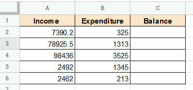
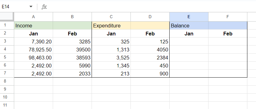
I have highlighted the following methods using the example dataset below to subtract the Expenditure value (column B) from the Income value (column A) and put the result or Balance in column C.
How To Subtract in Google Sheets Using a Simple Formula
A formula is a statement that a user makes to perform a calculation. A formula combines values and has one or more operations, like addition or subtraction.
The values used in a formula can be numeric or text references in a cell, such as a name. A formula can be simple with two variables and an operation, as shown below.
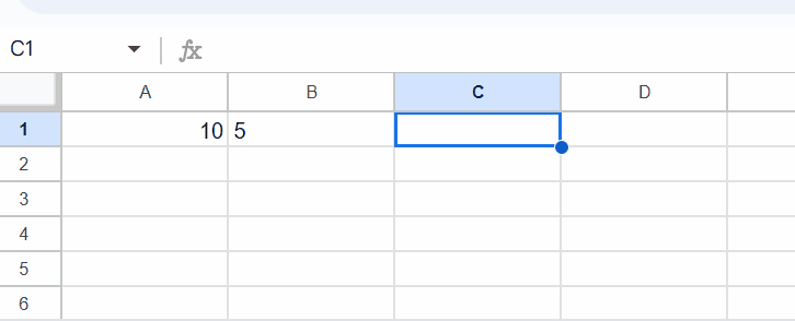
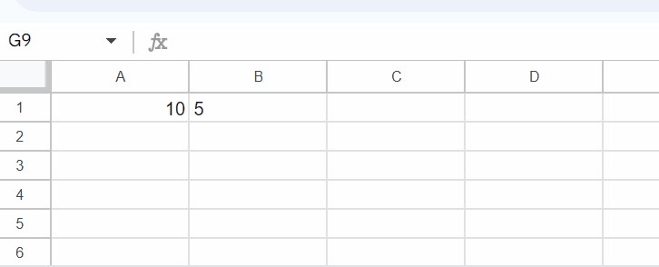
The easiest way to subtract in Google Sheets is to use the subtraction formula with the minus sign (-):
= 6 - 5
= A2 – B2
It can also be complex, consisting of a series of formula operators.
In any case, a formula should always start with an equal sign (=). Whenever you use a formula in a cell, it will be displayed on the formula bar.
When you finish entering the formula for subtraction in Google Sheets in a cell, it performs the operations as soon as you press the return key.
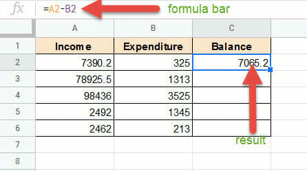
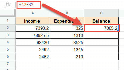
At this point, the result of the difference formula Google Sheets is displayed in the cell, while the actual formula is displayed in the function bar when the cell is selected:
To learn how to subtract in Google Sheets using the formula and following the steps below:
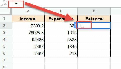
- Select the cell where you want the result to appear (cell C2).
- Enter the equal sign (=) in the cell to start the formula.
- If you look up at the formula bar, you will notice an equal (=) sign appearing there too.
- Select the cell containing the number you want to subtract from (cell A2).
- Enter a minus sign (-).
- Select the cell with the number you want to subtract, the subtrahend (cell B2).
- Press the “Return” key.
- The difference between the values in A2 and B2 should now be displayed as the result in cell C2.
- Once you have calculated with the first formula, getting the results for the remaining cells in the same column is easy.
- You will notice a small square at the bottom right corner of cell C2. This is called the Fill Handle. Hover your mouse over it.
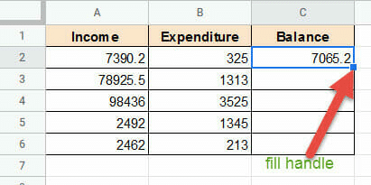
- When your mouse changes into a plus sign, double-click on the square.
- You will find the formula copied into all the cells in column C.
- Alternatively, you can drag the fill handle down the column till it reaches the last row.
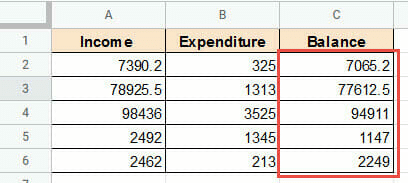
Each cell in column C should now contain the value of the corresponding Expenditure, subtracted from the Income!
Wasn’t that easy?
There’s more to come! Here’s another way…
How To Subtract in Google Sheets Using the MINUS Function
A function is a formula that has been pre-built to perform specific tasks. For example, there are functions to find sums, multiple, differences, and averages. MINUS is the Google Sheets subtract formula.
Like formulas, functions always start with an equal sign (=). The name of the function and parentheses follow this. If applicable, you can list parameters (or arguments) inside the parentheses.
Arguments, on the other hand, are input values that the function uses to perform its task. The number and type of arguments depend on the syntax of the function.
For example, Google Sheets has a function called MINUS that is used to subtract two numbers. This function’s syntax takes two parameters — the subtrahend and the minuend.
A standard subtraction equation will look like this:
8 - 6 = 2
In this example, the minuend is 8, and the subtrahend is 6.
If there is more than one argument, they are separated by commas. So, the MINUS function’s syntax is as follows:
=MINUS(value1, value2)
Here:
- value1 is the minuend.
- value2 is the subtrahend.
In this formula, value1 and value2 can be numbers, dates, or references to cells containing numbers and/or dates.
So, you can write either:
=MINUS(6, 5)
or
=MINUS(A1 , B1)
Like formulas, whenever you use a function in a cell, it is displayed on the formula bar.
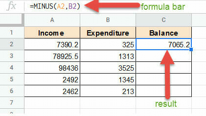
When you finish entering the subtract Google Sheet function in a cell, it performs the operations as soon as you press the return key.
At this point, the result of the subtraction function in Google Sheets is displayed in the cell, while the actual formula is displayed in the formula bar when the cell is selected:
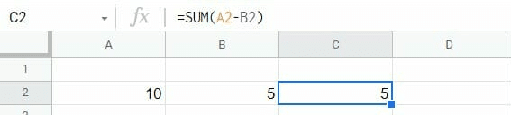
How To Subtract in Google Sheets With the SUM Function
Although the SUM function in Google Sheets is usually used when adding numbers, you can also use it for subtraction.
In this case, you use the minus symbol (-) with the parenthesis between the two values. You can use SUM as a subtract function Google Sheets like so:
SUM(A2-B2)
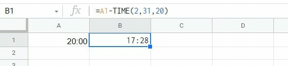
How To Subtract Time and Date In Google Sheets
Unfortunately, MINUS or SUM won’t allow you to subtract time effectively. Instead, you have to use the TIME function as well. You can do so with the following formula:
=cell reference-TIME(N hours,N minutes,N seconds)
Let’s look at an example so you can understand it better.
I want to subtract 2 hours, 31 minutes, and 20 seconds from the time in cell A1. The formula would be similar to this:
=A1-TIME(2,31,20)
Alternatively, you don’t need to use the time function in Google Sheets when subtracting dates. You can subtract them like normal values or use cell references.
For example, I can use the formula below to subtract the 7th of August from the 15th of January to know the number of days between the dates.
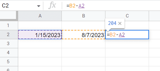
The result will be 204 days. If I want to change the format of this result, for example, changing it to months and days or even percentages, I can use the following steps:
- Select the cell.
- Go to “Format” > “Number.”
- Choose the appropriate format to use.
One thing to note is that the first day is usually not counted with any method for subtracting dates in Google Sheets. If you need the first day counted, you can add +1 to your equation.
How To Subtract Numbers in Google Sheets Using Arrays
The ARRAYFORMULA function is handy for fetching whole columns of data and completing calculations. Arrays also let you subtract columns in Google Sheets.
Here is how you would use an Array formula with the MINUS function:
=ARRAYFORMULA(MINUS(array1, array2)
Let’s substitute some figures into an example and see what it looks like:
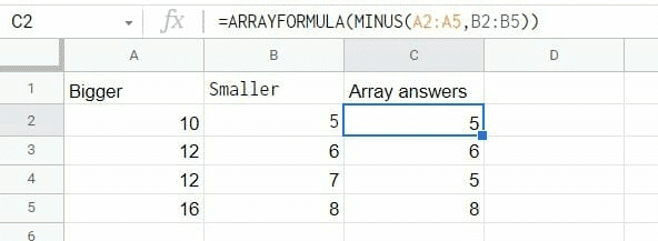
You can click and drag over the cell references rather than manually enter them.
How To Subtract in Google Sheets Across Multiple Worksheets
To subtract across multiple sheets, you must use the sheet prefix and a cell reference with the minus sign (-) in between. Here is an example:
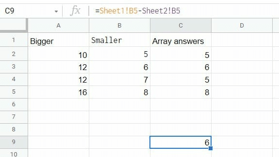
The above example has subtracted cell B5 in Sheet2 from B5 in Sheet1.
NOTE: It is imperative to add the exclamation mark (!) between the sheet name and the cell reference.
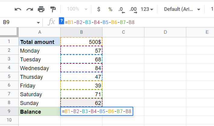
How To Subtract Multiple Cells in Google Sheets From the Total of One
It is also possible to subtract multiple cells in Google Sheets depending on how you want to subtract the values. You can subtract the cells in a sequence or linear form using the MINUS function.
For example, I can subtract all the values or cell references in one go to find the balance in the sheet below. This gives us a balance of $72.
You can also use the SUM function to subtract in the same example to subtract Google Sheets. You need to create the SUM formula and subtract the total value of that sum.
For example, in the spreadsheet example below, I used the sum of the values from B2 to B7 and subtracted it from the total with the formula:
=B1-SUM(B1:B8)
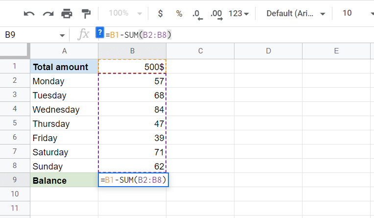
These two ways will give you the same answer, so choosing the most suitable method is up to you.
How To Subtract Matrices in Google Sheets
Sometimes, you may also find yourself with a set of data that requires you to subtract multiple columns from other multiple columns.
Rather than finding the difference cell by cell or column by column, you can do it all at once by subtracting matrices. This is done by using the Array formula.
Follow the steps below to learn how:
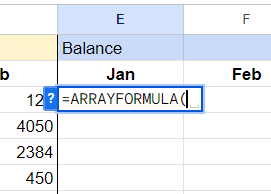
- Enter the equal sign (=) and ARRAYFORMULA in the first cell of the result matrix.
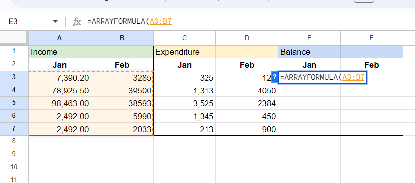
- Select the cells for the matrix you want to subtract from.
- In this case, it’s A3:B7.
- Add a minus sign (-).
- Select the cells of the matrix you want to subtract (C3:D7).
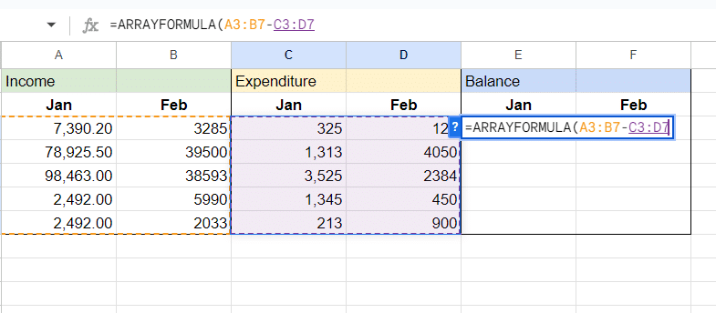
- Press “Enter” to see the results.
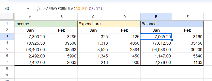
Here is the whole example formula:
=ARRAYFORMULA (A3:B7- C3:D7)
Using Subtraction Equations in Google Sheets
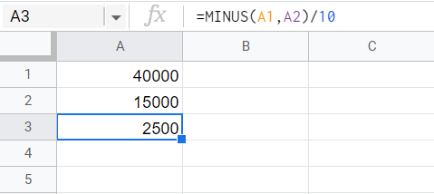
Sometimes, the function you want to carry out is not as simple as getting the difference between two values in Google Sheets. Therefore, you might use a more complex equation.
You can create subtraction equations using the MINUS function and other signs like divide (/), multiplication (x), and add (+). This is more convenient since you can combine multiple formulas to get one return much faster.
For example, in my example below, I subtracted the two values (40,000, 15,000) and then divided them by 10 to get the answer.
Frequently Asked Questions
How Do You Create a Subtraction Formula in Google Sheets?
There are multiple ways to create a Google spreadsheet subtraction formula. However, the simplest way is to use the MINUS function.
For example, to do the calculation 5-4, you would type the following formula:
=MINUS(5,4)
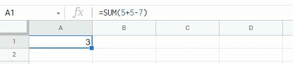
How Do You Add and Subtract on a Spreadsheet?
If you need to add and subtract in one formula, use the SUM function with the appropriate operators to signal to Google Sheets where to subtract and where to add.
Let’s say you wanted to find out 5 +5 -7. You could use the following formula:
=SUM(5+5-7)
How Do You Subtract Fractions in Google Sheets?
You can subtract fractions using the Google Sheet SUBTRACT formula alongside the MINUS function.
For example, to subtract one quarter away from one half, use the following formula:
=MINUS(1/2,1/4)
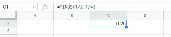
Alternatively, you can use cell references with the fractions instead of manually typing them. However, note that the results will be displayed as a decimal.
Related: How to Round Numbers
Wrapping Up Subtraction In Google Sheets
So now that you have learned how to subtract in Google Sheets using the various methods, you can familiarize yourself with formulas, making it easier to work in Google Sheets as your knowledge progresses.
I hope you found this article useful! You can also read more in our article on how to find absolute value in Google Sheets.
Other Google Sheets articles you may like: