Decimals in your data are a necessary evil. While it’s good to keep as many decimal places as you can (to ensure accuracy), it may make your spreadsheet difficult and sort of unappetizing to read.
Moreover, for the sake of uniformity and symmetry, it’s always a good idea to have all your data values rounded off to the same number of decimal places.
There are a few methods of how to round numbers in Google Sheets , and we are going to take a look at 5 of them in this tutorial.
Table of Contents
Different Rounding Functions in Google Sheets
There are a few different Google Sheets round function types, each of which serves a slightly different purpose. Depending on your requirement, you can choose anyone to round off your data values:
- ROUND
- ROUNDUP
- ROUNDDOWN
- MROUND
How Does Rounding of Numbers Work (The Logic Behind It)
The ROUND function takes a numeric value and rounds it to a specified number of decimal places, according to standard rules.
The standard rules of rounding are as follows:
- If the digit to the right of the digit to be rounded is less than five, then it remains unchanged. In the other words, the number is ‘rounded down’ to the nearest digit
- If the digit to the right of the digit to be rounded is greater than or equal to 5, then it is incremented by 1. In other words, the number is ‘rounded up’ to the nearest digit.
For example, when rounding off the number 1.263 to the second decimal place, the digit to be rounded is 6. The digit to the right of 6 is 3 (which is less than 5). So the digit to be rounded remains the same, and the final result after rounding is 1.26.
If instead, you are trying to round the number 1.267 to the second decimal place, the digit to be rounded is 6. The digit to the right of 6 is 7 (which is greater than 5). So the digit to be rounded is increased by 1 and the final result after rounding is 1.27.
How to ROUND Numbers in Google Sheets (using the ROUND function)
The syntax for the ROUND function is as follows:
ROUND(value, [places])
Here,
- value is the number that you want to round. This may be a numeric value or reference to a cell containing a numeric value.
- places is the number of digits or decimal places to which you want to round value. This parameter is optional. When it is not specified, its value is assumed to be 0 by default.
An Example Use Google Sheets to Round to 2 Decimal Places ( Or Any Other Choice)
Let us take a look at some examples of the round function Google Sheets uses to round the given values of column A to the number of places specified in column B, using the ROUND function:
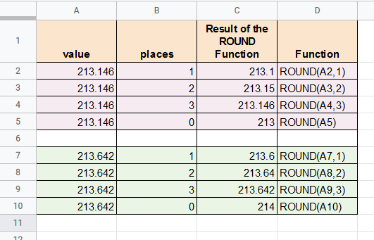
From the above image you will observe that Google Sheets limits decimal places like so:
- In row 2, we want to round off the value 213.146 to 1 decimal place. According to standard rounding rules, the rounding digit, 1 remains the same. So, the rounded number now becomes 213.1. We have essentially ‘rounded down’ the value 213.145.
- In row 3, we want to round off the value 213.146 to 2 decimal places. According to standard rounding rules, the rounding digit, 4 is increased by 1. The rounded number now becomes 213.15. We have essentially ‘rounded up the value 213.145.
- In row 5, there is no places parameter provided in the formula, so the default value 0 will be used. This means we want to round off the value 213.146 to 0 decimal places, in other words, to the nearest integer. According to standard rounding rules, the nearest integer to 213.146 is 213. Again, we essentially ‘rounded down’ the value 213.146.
- In row 10, there is again no places parameter. So we again need to round off the value to the nearest integer. The nearest integer to 213.642 is 214. Here, we essentially ‘rounded up’ the value 213.642.
Limit Decimal Places With Negative Values in Google Sheets
The ROUND function can also be used with negative values for the places parameter. In such cases, the value is rounded to the left of the decimal point. So,
- if places is -1, then the ROUND function will round the value to the nearest tens.
- if places is -2, then the ROUND function will round the value to the nearest hundreds.
- if places is -3, then the ROUND function will round the value to the nearest thousands.
and so on.
Check also: Limitations of Google Sheets
Let us take a look at a few more examples to understand how the ROUND function works with negative values for the place parameter:
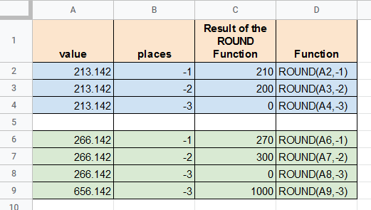
From the above image you will observe that:
- In row 2, we round off the value 213.146 to -1 places. The function removes all digits on the right of the decimal point. It then rounds the value to the left of the decimal point to the nearest tens. The nearest tens to the number 13 is 10. So, the function rounds down the value to 210.
- In row 3, we round off the value 213.146 to -2 places. The function rounds the integer portion of the value to the nearest hundreds. The nearest hundreds to the number 213 is 200. So, the function rounds down the value to 200.
- In row 6, we round off the value 266.142 to -1 places. The function rounds the integer portion of the value to the nearest tens. The nearest tens to the number 66 is 70. So, the function rounds up the value to 270.
- In row 9, we round off the value 656.142 to -3 places. The function rounds the integer portion of the value to the nearest thousands. The nearest thousands to the number 656 is 1000. So, the function rounds up the value to 1000.
It’s clear from the above examples that the ROUND function either rounds up or rounds down the given value, depending on the standard rounding rules. But what if you wanted to ensure that your value only gets rounded up and never down?
For such cases, you can make use of the ROUNDUP Google Sheets function.
How to Round Up in Google Sheets – The ROUNDUP Function
The ROUNDUP function works the same way as the ROUND function, except that it always rounds the value upward. This functions allows Google Sheets to roundup to the nearest one or any other choice you may have.
Syntax of the ROUNDUP Function
The syntax for the ROUNDUP function is the same as that of the ROUND function:
ROUNDUP(value, [places])
Examples using the ROUNDUP Function to Limit Decimal Places
Let us take a look at some examples to see how the ROUNDUP function works:
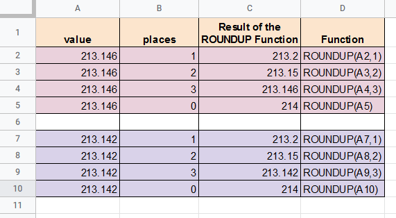
From the above image, it is quite clear that the ROUNDUP function always rounds up the value to the given number of decimal places.
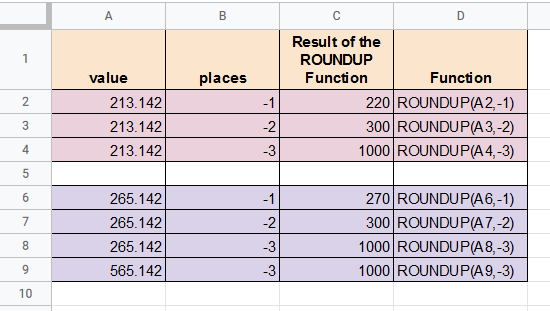
Similar to the ROUND function, the ROUNDUP function also supports negative values for the places parameter.
Here are some examples to help you understand how the ROUNDUP function works with negative values for the places parameters:
How to Round Down Numbers in Google Sheets
The ROUNDDOWN function works the same way as the ROUND function, except that it always rounds the value downward.
Syntax of the ROUNDDOWN Function
The syntax for the ROUNDDOWN function is the same as that of the ROUND function:
ROUNDDOWN(value, [places])
Examples using the ROUNDDOWN Function
Let us take a look at some examples to see how the ROUNDDOWN function works:
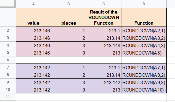
From the above image, it is quite clear that the ROUNDDOWN function always rounds down the value to the given number of decimal places.
Similar to the ROUND function, the ROUNDDOWN function also supports negative values for the places parameter.
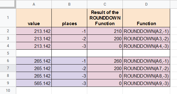
Here are some examples to help you understand how the ROUNDDOWN function works with negative values for the places parameters:
How to Round in Google Sheets to the Nearest Integer Multiple (MROUND Function)
Using negative values with the above rounding functions can help convert your numbers to the nearest multiples of 10, 100, 1000, etc. However, what if you want to convert values to the nearest multiple of some other number, like 2, 3, 15, etc.?
Google Sheets has something for that too. It lets you use the MROUND function. This function works the same way as the ROUND function, except that it lets you round a value to the nearest integer multiple of another value.
Syntax of the MROUND Function
The syntax for the MROUND function is similar to that of the ROUND function:
MROUND(value, factor)
Here,
- value is the number you want to round.
- factor is the number to whose multiple the value will be rounded.
Unlike ROUND, ROUNDDOWN, and ROUNDUP functions, you cannot use negative values in the second parameter of the MROUND function, unless the first parameter is also a negative number.
Examples using the MROUND Function
Let us take a look at some examples to see how the MROUND function works:
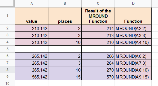
From the above image you will observe that:
- In row 2, the MROUND function rounds the value 213.142 to the nearest multiple of 2. So, we get the result as 214.
- Similarly, in row 9, the MROUND function rounds the value 565.142 to the nearest multiple of 15. So, we get the result as 570.
In this tutorial, we showed you how to round numbers in Google Sheets using four different rounding functions in Google Sheets. These included the ROUND, ROUNDUP, ROUNDDOWN, and MROUND functions.
The ROUND function can help you round values according to standard rules, while the ROUNDUP function ensures that your values always get rounded upwards. Similarly, the ROUNDDOWN function ensures that your values always get rounded downwards.
The MROUND function, on the other hand, lets you round values to multiples of a certain integer.
Using the CEILING Function in Google Sheets to Round Numbers
You can also use the CEILING function to round up numbers in Google Sheets to the nearest 1 or any other specified place.
The syntax for the CEILING function goes as follows:
=CEILING(Number, Significance)
In this syntax:
- Number is the number you want to round (usually a cell reference)
- Significance is the decimal place value that you wish the number to be rounded up to
Check out the below example
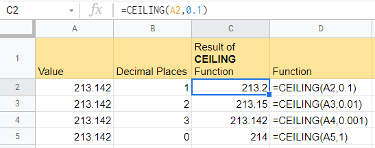
As you can see to show the result to one decimal place the significance is set to 0.1, which means the result will be shown in multiples of 0.1
A similar approach is taken to show results in multiples of 0.01, 0.001, and 1. You could also use the CEILING function to round up into multiples of 10s, 100s, 1000s etc.
Which Google Sheets Round Function Should You Use?
Once you know what each rounding function does, applying them according to your needs becomes second nature. Just think about whether you need to round up, down, or to the nearest figure.
We hope this tutorial has enabled you to understand the differences between each of the rounding functions and now you know how to round numbers in Google Sheets.
Other Google Sheets tutorials you may like: