How To Multiply in Google Sheets and Excel

To multiply in Google Sheets and Excel, use the equal sign followed by a multiplication formula. After all, most people use Google Sheets for two basic purposes — creating a record database or doing simple calculations, such as multiplying cells or columns.

In fact, there are many ways to multiply columns (or cells or numbers) in a spreadsheet. And they’re usually platform agnostic. That means you can use the same method to multiply in Google Sheets that you would in Excel. I’ll show five examples below.

Multiplying Two Numbers in Google Sheets

If you have two numbers or cells that contain the numbers that you want to multiply, there are a couple of techniques to carry out multiplication on Google Sheets. There are two Google Sheets multiplication formulas that you can use: Multiply and *.

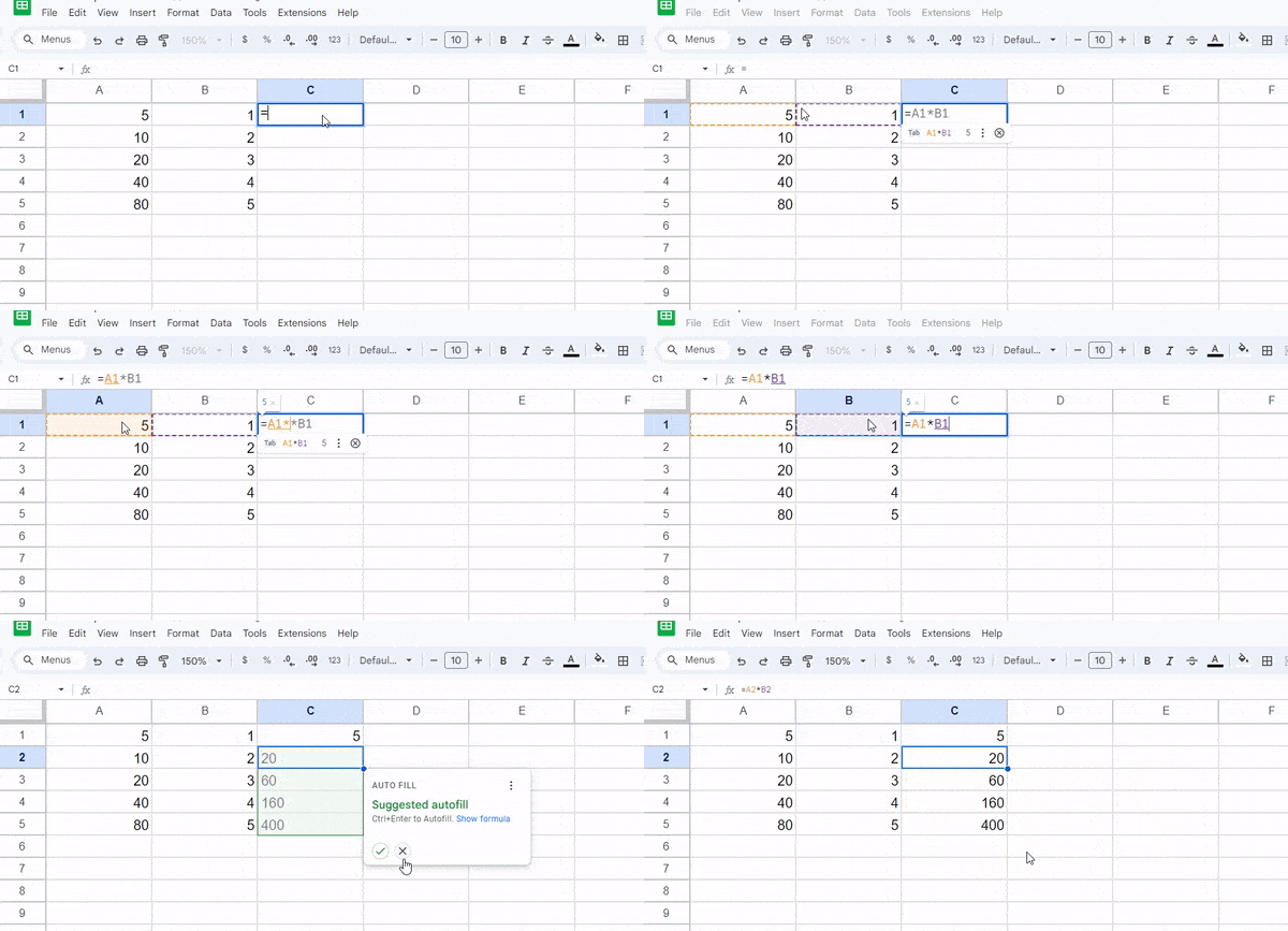
This animation shows how you can also use the auto-fill to multiply all rows in a data range. That saves time, especially when you’re working with large data sets.

How To Multiply in Google Sheets Using the MULTIPLY Function

Since multiplying numbers is such a common task, Google decided to build a dedicated Google Sheets MULTIPLY formula in its system, (and in case you were wondering, it’s not MS Excel).

Suppose you want to multiply two numbers, for example, 12 and 14, here’s how to multiply in Google Sheets:

1. Type the equals sign (=) in the cell
2. Type MULTIPLY or select it from the formula suggestion
3. Type in the two values (cell references) separated by a comma (,)
4. Close the bracket and click “Enter“

You can use the Google Sheets multiplication formula below:

=MULTIPLY(12,14)

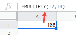
This MULTIPLY formula in Google Sheets is a great method to use when you only have two numbers and you want to get the resulting value quickly.

Additionally, you can also use the cell references instead of the values. For example, if cell A1 has a value of 12 and A2 has a value of 14, here is how to multiply in Google Sheets using the cell references:

1. Type the equals sign (=) in the cell
2. Type MULTIPLY or select it from the formula suggestion
3. Select the first cell reference (A1) then type a comma (,)
4. Select the second cell reference (A2)
5. Close the bracket and click “Enter“

You will end up with the Google Sheets multiplication formula below:

=MULTIPLY(A1,A2)

While the MULTIPLY sheets formula is quick and easy to use, it can only be used with two values. Therefore, if you have more than two values and try to use this formula, it will give display an error.

How To Multiply in Google Sheets Using the Multiply Operator

You can also use the multiply operator (an asterisk sign *) to multiply two or more cells or numbers in Google Sheets.

For example, if you want to multiply two numbers, such as 12 and 14, you can use the following method:

1. Type the equals sign (=) in the cell
2.  Type in the two values separated by an asterisk (*)
3. Close the bracket and click “Enter“

You will end up with the formula below :

=12*14

If these values are in cells A1 and A2, you can use the formula below:

=A1*A2

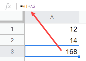
When using the multiplication operator, you can multiply more than two values. Simply use the multiply operator between all the values that you want to multiply. You can also use the multiplication operator to square numbers in Google Sheets.

For example, if you have values in cell A1, A2, and A3, you can use the formula below:

=A1*A2*A3

NOTE: If any of these cells are empty, the formula will give you 0.

One important thing to know when using a multiplication operator is to follow the order of precedence. For example, if you use the formula below, it will give you 170 (as it first does the multiplication and then adds the 2 to the result):

=12*14+2

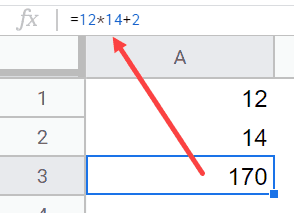
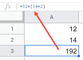
If you want to add 2 and 14 first and then multiply, you need to use the  following formula (where brackets are used to separate the section that is calculated first:

=12*(14+2)

Related: How to Divide in Google Sheets

How To Multiply Columns in Google Sheets

While the above examples dealt with multiplying single values or cells, in this section, I will show you how to use Google Sheets to multiply two columns (or more) with a simple formula.

For example, if you have a dataset similar to below and you want to get the multiplied value of cells in column C, use the following formula:

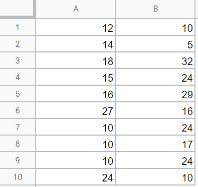
1. Type the equals sign (=) in the adjacent cell to the first row of data
2. Type the ARRAYFORMULA or select it from the formula suggestion
3. Select the first column range (A1:A10)
4. Type in the asterisks (*)
5. Select the second column range (B1:B10)
6. Close the bracket and click “Enter“

You will end up with the following formula:

=ARRAYFORMULA(A1:A10*B1:B10)

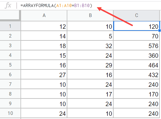
Since this is an array formula, you only need to enter this in cell C1 and it will automatically fill in the data for the rest of the column cells.

Also, with array formulas, you can not delete or edit a part of the resulting array. However, you can delete the entire array.

You can also use the formula below to first multiply the cells in the row, and then copy the formula for the cells in the column.

Since the above is not an array formula, you can change or edit individual cells that you want.

In case you want to get the sum of all the multiplied values in a single cell, you can use the SUMPRODUCT formula:

=SUMPRODUCT(A1:A10*B1:B10)

Note that this is pretty similar to when you want to sum a column. Just make sure you’ve got the whole range included in your formula.

Tips for Multiplying in Google Sheets

• Check your formulas: If you have a wrong result, it’s likely you’ve mistyped a part of the function. So remember to double-check everything and ensure the formula is correct.
• Review the operators: The multiply operator is an asterisk sign (*). Therefore, you should not use any other symbol except for brackets.
• Choose the result cell carefully: Make sure you’ve selected the right cell that you want to show the result. The same goes for selecting an appropriate column.
• Use cell references: Once you wrap your head around the cell references, it will save you a lot of time compared to writing the formula out manually.

Frequently Asked Questions

Can You Multiply Data Across Multiple Rows Without Entering a Formula in Every Row?

Yes, you can multiply across multiple rows. The Google spreadsheet multiplication formula used across multiple rows is the ARRAYFORMULA.

For example, if you want to multiply rows 1-5 in columns A, B, and C. You could use the following array formula:

=ARRAYFORMULA(A1:A5*B1:B5*C1:C5)

The colon in between the cell references indicates the cell range while the asterisk sign (*) is used as the Google Sheets multiplication operator.

This will give you results in the entire column. Then, you can simply use the SUM formula to get a grand total.

What Is the Formula to Multiply in Google Sheets?

MULTIPLY is the aptly named multiplication function in Google Sheets. For example, if type you type the formula below, you will get a result of 10:

=MULTIPLY(2,5)

Alternatively, you can use the asterisk (*) operator instead:

=2*5

How Do I Multiply More Than Two Numbers in Google Sheets?

If you want to multiply two numbers or more, there are two methods:

1. Use the asterisk operator (*), like so: =2*3*4*5
2. Use multiple MULTIPLY formulas
   

Wrapping Up

So, how to multiply in Google Sheets? As you can see, there are multiple ways to multiply in Google Sheets. Depending on whether you want to multiply cells or columns, you can choose from the MULTIPLY function in Google Sheets or use the asterisk operator.

We hope you have found this tutorial helpful. Feel free to share your thoughts on how to multiply in Google Sheets in the comments below!

Related:

• • Google Sheets Percentage Formula (5+ Easy Examples)
  • How To Number Rows in Google Sheets (Add Serial Numbers)
  • How To Count Cells with Specific Text In Google Sheets
  • How To Square In Google Sheets
  • Convert Formulas to Values in Google Sheets
  • How To Subtract in Google Sheets
  • How To Calculate Weighted Average In Google Sheets