How to Filter By Color in Google Sheets (Using a Formula)

There are some times I wish Google Sheets had some more functionalities like MS Excel.

One such functionality that isn’t available in Google Sheets is the ability to filter by color.

For example, suppose I have a dataset as shown below and I want to filter all the rows where the record has been colored in a specific color.

Unfortunately, there is no direct way to filter by color in Google Sheets.

But there are a few indirect ways

In this tutorial, I will show you a couple of methods you can use to filter rows based on the color as the criteria in Google Sheets.

Using Google Apps Script to Filter by Color

Suppose you have a dataset as shown below and you want to filter all the rows where the cells have been colored.

For Google Sheets to filter a dataset, it needs to be able to use criteria in the cells. By using this criterion, it filters all the records that match the criteria.

And since the color is not a value by itself, we can not filter based on it by default.

By using a Google Apps Script, you can convert the color into a HEX code (which is a code assigned to each color).

Once you have the HEX code, you can now filter the data based on it.

Below is the script that will create a function in your Google Sheets document that you can use to get the HEX code of the color that has been applied to the cells.

function GetCellColorCode(input) 
{ 
var ss = SpreadsheetApp.getActiveSpreadsheet(); 
var cell = ss.getRange(input); 
var result = cell.getBackground(); 
return result 
}

The above function takes the range as input and returns the background color hex code of the input cell/range.

Once you have added this code to the Google Apps Script Editor, you will be able to use the function ‘GetCellColorCode’ to get the HEX code of the cell color in a separate cell.

How to add the code to the Google Script Editor is covered later in this section.

Let me first show you how this formula works.

Enter the following formula in the adjacent column of the dataset

=GetCellColorCode("A"&ROW())

The above formula uses the function we created (GetCellColorCode) and inputs the range such as A2 or A3 or A4 – depending on the cell.

Since I didn’t want this to be manual, I have used “A”&ROW() – which returns the cell address based on the row in which the formula is used. In row 2, this would return A2, in row 3, it would return A3, and so on.

Once you enter this formula for all the records, you will get a result as shown below:

The cells that have no color return the hex code #ffffff and the cells that have a color return the hex code of that color.

Now that you have the hex codes in a separate column, you can easily filter by color by actually filtering by hex code value.

Below are the steps to filter all the rows where the color is yellow in the above dataset:

1. Select any cell in the dataset
2. Click the Data tab
3. In the options that appear, click on ‘Create a Filter’. This will add filters to all the header cells in the dataset (a downward pointing arrow icon will appear at the right of each header cell).
4. Click the Filter icon for the ‘Hex Code’ column
5. In the filter options that appear in the box, deselect all color hex codes and select the one based on which you want to filter the dataset.
6. Click Ok.

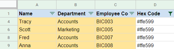
This will filter the rows based on the selected color hex code (as shown below).

A few things to know about using the custom formula created using the script:

1. This function is only available to the Google Sheet document in which you have added the script. It will not be available in any existing or new Google Sheets document. If you want it to use in other documents, you need to add it there as well.
2. This formula is not dynamic. This means that if you change the color of any cell, the formula would not update automatically. Sometimes, it doesn’t even update when you refresh the Sheet. The best way would be to use the formula in a new column and delete the existing one.

How to Add the Script to Google Script Editor

Below are the steps to add the script to filter by color in the Google Sheets script editor:

1. Copy the above script code
2. Click on Tool tab
3. Click on Script Editor
4. In the Script editor that opens, paste the code in the Code.gs window (you can delete any pre-existing code there if you don’t want it)
5. Click on the Save button in the toolbar
6. Close the Script editor.

The above steps add the code to create a function to filter by color to that specific Google Sheets document.

Now you can use the function that you have created in any of the worksheets in the Google Sheets document.

Note: When you create a custom function, Google Sheets does not show you the function name in worksheets when you type the first few alphabets of the function name. You need to know the exact name of the function and the inputs it takes to make it work.

You may also like the following Google Sheets tutorials:

• How to Delete Empty Rows in Google Sheets
• How to Insert CheckBox (Tick Box) in Google Sheets
• How to Transpose Data in Google Sheets
• Google Apps Script for Google Sheets – Easy Beginner’s Guide
• How to Color Alternate Rows in Google Sheets
• How to Hide Columns in Google Sheets
• How to Count Cells with Specific Text in Google Sheets
• FILTER Function in Google Sheets