Alternate Row Color in Google Sheets: Simple Guide

Watch Video – How to Color Alternate Rows in Google Sheets (With and without Conditional Formatting)

If you prefer reading over watching a video, below is a written tutorial for Google Sheets alternate row color.

Google Sheets has been adding some awesome features lately. Things that used to take a lot of time and know-how can now easily be done with a few clicks.

And one such thing is to color alternate rows in Google Sheets.

Now, there’s an added functionality in Google Sheets that makes it super easy to have Google Sheets highlight every other row. Earlier, you had to use conditional formatting to get this done, but now it can be done in two clicks (both methods are covered in this tutorial).

In this tutorial, I will show you how to apply alternating colors in Google Sheets and the conditional method in case you want to color every third or fourth row.

Let’s get started!

How to Color Alternate Rows In Google Sheets

Here’s how to alternate colors in Google Sheets:

1. Select your data range
2. Got to Format > Alternating colors
3. Select a color scheme from the default styles or customize your own
4. Click Done.

As you can see, it is a straightforward process. Suppose you have a dataset as shown below, and you want to highlight/color every alternate row in this dataset:

Below are the steps to have Google Sheets make every other row gray:

1. Select all the cells in the dataset (including the header)
2. Click the ‘Format’ tab
   

   

3. Click on ‘Alternating’ colors
   

   

4. In the Alternating colors pane that opens on the right, make the following changes/selections:
   • In the Styles option, make sure the ‘Header’ option is selected. in case your data set doesn’t have headers, deselect this option
   • Select from any of the pre-made templates, or specify custom colors for Header, Color 1, and Color 2

The above steps would instantly highlight every other row in the dataset (as shown below).

To remove the Alternating color, select any cell in the dataset, click the Format tab and then click on the ‘Alternating colors’ option. This will open the pane where you have the option to ‘Remove alternating colors.’

A few things to know when using the ‘Alternating colors’ functionality in Google Sheets:

• In case you already have some color applied to the cells, these will be overwritten by the ones you choose when highlighting using the ‘Alternating colors’ functionality. And when you remove the alternating colors (steps mentioned in the yellow box above), it will remove the alternate colors while keeping the original colors intact
• In case you want to change the color of the header or any specific cell or range, you can do that manually. It will simply overwrite the existing colors.
• If you expand the dataset and add more records at the bottom, Google Sheets will automatically highlight the alternate rows in the colors you specified. However, in case you delete records, the colors would stay, and you would have to manually remove these.
• If you insert additional rows in the dataset, Google Sheets will automatically adjust the coloring.

Related: How to Lock Cells in Google Sheets

Google Sheets Alternate Row Color for Every Third, Fourth, Etc Row

For highlighting/coloring alternate rows, the method shown above is the best and fastest.

But what if you don’t want to color every other row? What if you want to color every third row or every fourth row?

In that case, you can’t use the ‘Alternating colors’ functionality of Google Sheets. You need to use Conditional Formatting with a simple formula.

Conditional formatting is used to format cells in your sheet based on conditions, for example, filtering by color or showing negative numbers in red.

Suppose you have the following dataset, and you want to highlight every third row in this dataset:

Below are the steps to use Conditional Formatting to color every third row in Google Sheets:

1. Select the dataset for which you want to color every third row (excluding the header)
2. Click the ‘Format’ tab
   

   

3. Click on the ‘Conditional formatting’ option. This will open the Conditional Formatting pane on the right
   

   

4. In the Format rules drop-down, click on the ‘Custom formula is’ option (you need to scroll down the list to get this option)
   

   

5. In the ‘Value or Formula’ field below it, enter the following formula: =MOD(ROW(),3)-1=0
   

   

6. Specify the formatting style. You can color every third row or can make it bold, italicize it, apply strikethrough format, etc.
   

   

7. Click on Done

The above steps would apply the specified format/color to every third row in Google Sheets (as shown below).

How does this work?

Now let’s understand how this works.

The entire magic is in the below formula:

=MOD(ROW(),3)-1=0

The above formula uses the ROW function to get the row number of each cell. This row number is then used in the MOD formula.

MOD formula divides the given number with the specified divisor (which is 3 in our example) and gives us the remainder. So for the second row, the formula becomes

=MOD(2,3)-1=0

So for the second row, the MOD formula returns 1, which is not equal to 0. So the first row in our dataset returns a FALSE.

Similarly, the second row would also return a FALSE, and the third row will return a TRUE.

The same logic is applied to all the cells, and only the ones in every third record will return TRUE.

And since Conditional formatting only applied the specified format to those cells for which the formula returns TRUE, every third row gets highlighted in the specified format.

The reason I have subtracted 1 from the MOD formula is that I am starting from the second row onwards.

You can use the same logic to highlight every fourth row in Google Sheets by using the below formula:

=MOD(ROW(),4)-1=0

Note: You can also use the same logic to highlight alternate rows as well, however, since Google Sheets has an in-built functionality for alternating rows, it’s best to use the inbuilt one.

In case you don’t edit the formatting or want to delete it, click any of the cells in the dataset (that has the formatting applied), click on Format and then click on Conditional Formatting. This will open the conditional formatting pane where you can edit the rule or delete it.

You can copy and paste the conditional formatting, just like you can copy and paste values or formulas. To do this, copy the cells/range where conditional formatting is already applied and copy it. Go to the cells where you want to apply it, right-click and then go-to Paste Special and click on Paste Formatting only.

How to Alternate Colors for Columns

You can also apply alternating colors to columns instead of rows in Google Sheets. To do this, you will need to use conditional formatting with the formulas =ISEVEN and =ISODD. Here’s how to do alternating colors in Google Sheets for your columns:

1. Select your data range

2. Go to Format > Conditional formatting

3. In the conditional formatting window, click +Add rule.
4. In the formatting rules, choose Custom formula is

5. Type in the formula =ISODD(COLUMN()) if you want the first column to be colored or =ISEVEN(COLUMN()) if you want to start the color from the second column

.

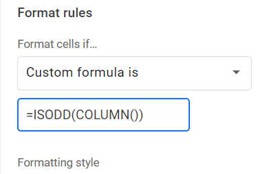
6. Choose the color and style
7. Click Done

How to Apply Dynamic Alternating Colours

Dynamic sheets are sheets that are constantly changing. If you use the Alternating color option to apply Google Sheets alternating row colors, then you will have to keep doing it every time you update the data in your sheet.

Instead of all this work, you can simply create dynamic alternating colors for your data range.

To do this, you will have to use conditional formatting instead of Alternating colors. Here’s how to color every other row in Google Sheets using dynamic alternating colors:

1. Select all the columns in your range

2. Go to Format > Conditional formatting

3. In the conditional formatting window, click +Add rule.

4. In the formatting rules, choose Custom formula is:

5. Input the following formula:

=AND(NOT(ISBLANK($A2)),ISODD(ROW()))

For the range in ISBLANK, you will need to put the first cell of your data range.

6. Choose the color you want for your alternating rows

7. Click Done.

If you add another row of data to you’re range, you won’t see any change.

However, if you add two more rows, the rows will automatically apply the dynamic row colors.

Conclusion

In this article, we have shown you a couple of ways to highlight every other row in Google Sheets, create dynamic alternating rows, and how to apply alternate colors to columns.

We hope you found this tutorial for Google Sheets alternate row color useful.

Related:

• How to Delete Empty Rows in Google Sheets
• How to Change Row Height In Google Sheets
• How to Wrap Text In Google Sheets
• How to Insert Multiple Rows in Google Sheets
• How to Freeze Rows in Google Sheets
• How to Group Rows and Columns in Google Sheets