The Complete Google Sheets Checkbox Guide

To add a checkbox in Google Sheets, use the “insert” menu and choose the “checkbox” option. I’ll discuss more ways to use the check box (also called a tick box) below. My guide also discusses how to add a checkbox in Excel and how to duplicate checkboxes so you don’t need to use the menu every time.

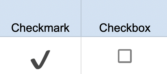
How a Checkbox in Google Sheets Differs from a Checkmark

You can easily create dynamic lists and charts where the user can simply click on the checkbox and program your data/charts to update. But before I get into the mechanics of inserting and using a checkbox/tick box in Google Sheets, let me quickly cover the difference between a checkbox and a checkmark.

A Google Sheets checkmark is a symbol that you insert as text within the cell. It doesn’t have any interactivity and can be used merely as a symbol or a bullet point. You can have text before or after a checkmark. It’s a formatting tool.

A checkbox, on the other hand, is interactive. While it is confined to a cell, you can click on it and it will change the state. So if it’s unchecked and you click on it, it will be checked (and vice versa). According to the U.S. Web Design System (USWDS), checkboxes are a fundamental part of modern web design.

Note that you can not have any text before or after a checkbox (tick box) in Google Sheets. You can only have the checkbox and nothing else.

How To Insert A Checkbox In Google Sheets

Let’s take a look at an example Sheet where we want to include check boxes. Remember, these are interactive cells. You can click the box to tick it and click again to untick it. Here’s what that looks like in Google Sheets.

To add these types of checkboxes, select where you want to include them in your sheet. Then, go to the Insert menu at the top of the window. In that menu, click “checkbox”. It automatically adds the interactive box into whichever cell or cells you had highlighted.

Here’s what the menu looks like:

1. Select the cell or cells in which you want to insert the Google Sheet checkbox  (tick box)
2. Click the ‘Insert’ option
3. Click on the ‘Checkbox’ option.

The above steps would insert a checkbox in the selected cell. In case you have selected multiple cells, checkboxes will be added to all the selected cells. Note that in case you have any text or formula in a cell and you insert a checkbox in it, Google Sheets will remove the text/formula and replace it with the checkbox.

Video Guide on Adding a Checkbox

Prefer to watch how it’s done? Here’s my video on how to add a checkbox in Google Sheets.

How to Add a Checkbox in Excel

In Microsoft’s Excel, the process is pretty similar. To add a checkbox in a worksheet, just click the developer tab. Then click “format” and choose the check box.

1. Click the developer tab.
2. Click format.
3. Choose the tick box.
4. Choose the cell where you want it to appear.

Unlike in Google Sheets, you can add text to a cell with a check box in Excel.

Formatting a Check Mark on Google Sheets

Now that you know how to insert a checkbox in Google Sheets, the next step is to format it. Since a checkbox is a part of the cell, you can format it just like any other cell.

For example, you can apply a color to the cell, and the checkbox will change the color from gray to the selected color. Similarly, you can also change the font in case you want bigger checkboxes. One common formatting choice is conditional formatting. That way, you could automatically highlight any checked cells in green.

Sort and Filter

Adding color to tick boxes is easy with conditional formatting, but that’s not the only way to sort data. Since the checkbox is a part of the cell, you can sort and filter them.

For example, if you have a list of tasks with checkboxes in adjacent cells, you can select the entire range and sort the list alphabetically. This will also sort the checkboxes in the selected range. That’s how I built my task list templates.

Creating a Google Sheets True & False Checkbox

It might sound strange, but check boxes in Google Sheets are either TRUE or FALSE:

• If the check box is checked, the value is TRUE
• If the check box is unchecked, the value is FALSE

You can see this yourself by selecting any cell with the checkbox and looking at the formula bar).

You can use these TRUE/FALSE values in the formulas. For example, I can list items and use the checkbox to mark an item as complete. I can also count the total number of completed items by simply counting the value of “TRUEs” in the list.

You can do some valuable things when you add a checkbox in Google Sheets::

1. Create a to-do list and mark tasks as done/complete.
2. Highlight specific data points based on selection (e.g., Top 10).
3. Create interactive charts in Google Sheets.

So let’s cover a few examples. These are some of the most powerful ways to use checkboxes in Google Sheets.

1. Add Checkboxes for Interactive To-Do Lists

It’s easy to use checkboxes to create a to-do list. As soon as you click on these boxes, it will mark the item as complete.

When the checkbox is clicked, the value in the cell becomes TRUE. If the value is FALSE, the format won’t be applied.

Here, I’ve used conditional formatting to highlight the TRUE value in green and apply strikethrough formatting.

1. Enter the tasks/items in column A and insert checkboxes in column B (in adjacent cells).
2. Select the cells in Column A
3. Select Format > Conditional Formatting in the dropdown menu.
4. Click ‘Format cells if‘ > ‘Custom formula is‘.
5. Enter the following formula: =$B2 (which selects all of the checkbox cells).
6. Specify the format (color and the strike-through format).

2. Highlighting Data with Check Box Functionality

You can use the checkbox to make your reports more visually appealing and easier to read.

In this example, Google Sheets will highlight the data in the table once you select any checkboxes:

This example’s conditional formatting is dependent on the value of the cell with the checkbox.

In the above example, if I select the checkbox for “>85”, it instantly changes the color of the cells in Column B that are greater than 85.

1. Add the checkbox (and specify the criteria for it as text in the adjacent cell)
2. Select the cells in Column B (with checkmarks).
3. Select Format > Conditional Formatting > Format cells if
4. Click on ‘Custom formula is’ option and enter the following formula: =AND($E$3,B2>=85)
5. Specify the format when marks are more than 85 (I’ve used green in my example).
6. Click Done.
7. Click Add New Rule > Format cells if > Custom formula is
8. Enter the following formula: =AND($E$4,B2<35)
9. Specify the format when marks are less than 35 (I’ve used red in my example).
10. Click Done.

The AND function (used in the steps above) checks for two conditions:

• Whether the cell with a checkbox is checked or not (i.e. if checked the value is TRUE)
• Whether the cell has a value that meets the criteria (i.e., greater than 85 or less than 35)

When both of these conditions are met, the cells are highlighted based on their values.

3. Create Dynamic Charts using Checkboxes

Charts derive their values from the cells in the spreadsheet, and checkboxes contain values. That means we can use checkboxes to affect the appearance of our charts. Neat, right?

That means we can create charts that show dynamic values. You can update or change a chart based on whether a checkbox is checked or not. That means you can create a dynamic chart in Google Sheets. Here’s how.

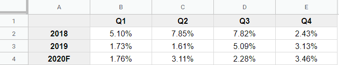
Below, I have a dataset that shows the profit margin values of a company over three years.

I can use the above dataset and combine it with the checkbox functionality to create a chart:

These types of charts are useful for multiple data series, as well as showcasing the data most useful for end users.

Note that I’ve created a dynamic dataset that only shows values when the corresponding checkbox is checked. If the checkbox isn’t checked, it won’t show the data – and the chart won’t show the line for it either.

I’ve created a copy of the original dataset, but this copied dataset is simultaneously dependent on the checkbox cell value. If you’ve checked the 2019 checkbox, 2019’s data will be populated in a dynamic second dataset. Otherwise, it will appear blank.

The first step is creating a second dataset that’s dependent on the checkboxes.

2018’s Data:

 =B2

I’ll need all of the original data points, as these will always be visible in the chart. In this example, I’ve used a simple reference to the original data.

2019’s Data:

=IF($H$3,B3,"")

The IF formula checks whether the checkbox in cell H3 is checked or not. If it’s checked, it returns TRUE and the original data point will be returned by the IF formula. If the checkbox is unchecked, the cell H3 returns FALSE (and the IF formula returns a blank cell).

Blank cells aren’t plotted in the chart. Therefore, you won’t see anything in the chart when the checkbox for that series is unchecked.

For 2020 Data

=IF($I$3,B4,"")

The same logic works for the 2020 data series. It is dependent on the checkbox in cell I3.

Once you have a new dataset that’s dependent on checkboxes, you can use this to create the chart.

In this example, I used a combination chart in Google Sheets, where:

• the 2018 value is shown as columns
• 2019 and 2020F values are shown as lines.

How to Use Data Validation to Add Custom Values to Checkboxes

You can use the checkboxes to indicate values:

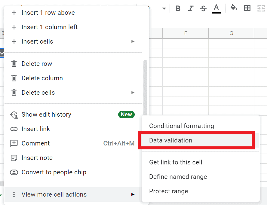
1. Right-click on the cell with the checkbox
2. Navigate to More cell actions > Data validation
   
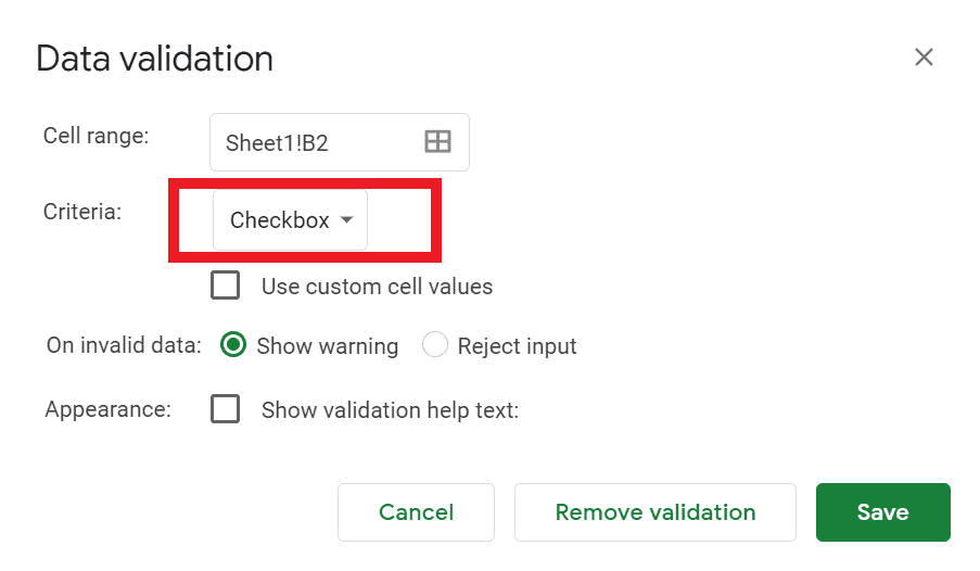
3. Make sure the value in the Criteria dropdown menu is set to Checkbox
   
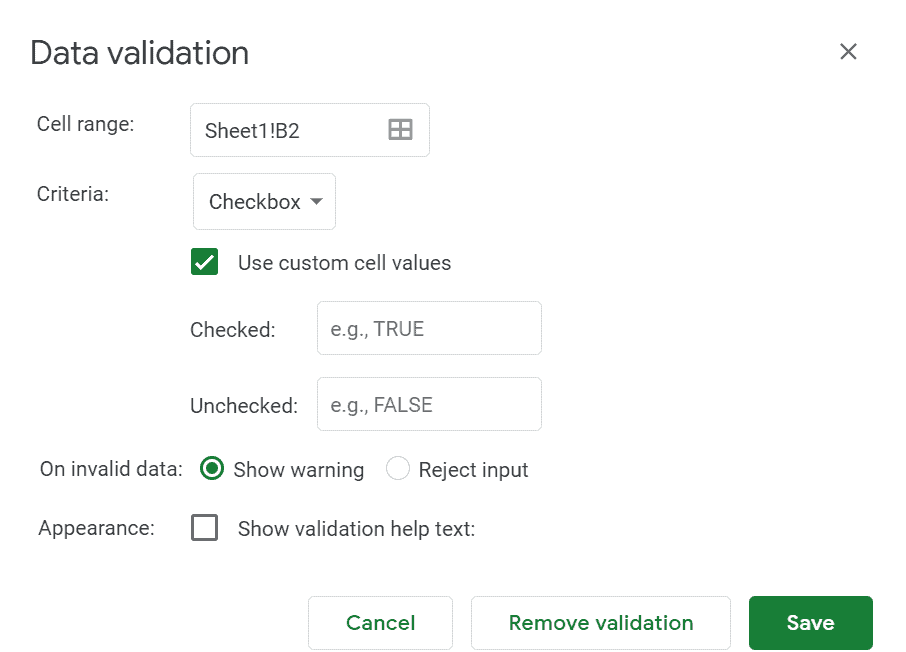
4. Check the “Use custom cell values” box. input the values you prefer (e.g., color, font). Click “Save.”
   

How to Remove Custom Values from Checkboxes

To remove custom values, follow the same steps for adding them – but uncheck the “Use custom values box.”

Can Google Sheets Add a Checkbox in the Mobile App?

Yes, it’s possible to use Android and MacOS. To make a check box in the Google Sheets app:

1. Select the cells you want to add checkboxes to
2. Tap the three dots menu
3. Select Data validation
4. In the criteria dropdown, select the checkbox option.

Note that Google’s support also talks about adding checkboxes in Google Docs.

How to Copy and Delete Google Sheets Checkboxes

Google checkboxes can be copied and pasted like any other regular cell. To delete a checkbox from a cell (or a range of cells), simply select the cells and hit the Delete key.

Note: If you select a cell that has a Google Sheets checkbox and type something in it, the new text will replace it.

Ideas to Format Check Boxes in Google Sheets

Since a checkbox is a part of the cell, you can format it just like any other cell. For example, you can use conditional format rules to apply a color to the cell, changing the checkbox from gray to the color of your choice. You can also change the font in case you want bigger checkboxes.

Say that you have a list of tasks with checkboxes in adjacent cells. You can select the entire range and sort the list alphabetically. This will also sort the checkboxes in the selected range.

Frequently Asked Questions

As always, I’m including some of the most common questions I hear on the subject. Please take a look and let me know in the comments if I missed anything!

What’s the Difference Between a Checkmark and a Checkbox?

There’s a slight difference between a checkmark and a checkbox:

• A Google Sheets checkmark is a symbol inserted as text within cells. It doesn’t have any interactivity and can be used as a symbol or a bullet point.
• A checkbox is interactive and confined to a cell. In Google Sheets, a checkbox cannot have any text before or after it.

Can You Put a Checkbox and Text in the Same Cell in Google Sheets?

No, you can’t. A tick box takes up the entire cells and basically contains a value of TRUE or FALSE. You cannot add any other data to the same cell, but you can modify your formatting to make it look like there’s text in the same cell.

How Do I Tick Multiple Checkboxes in Google Sheets?

Highlight the cells and press the space bar to tick or untick cells in bulk.

Can You Make a Checklist in Google Sheets?

Yes, once you have a list of items, highlight the adjacent cells and navigate to Insert > Checkbox to add them.

How Do I Use Checkboxes in Conditional Formatting?

Say that you have a checkbox in B2 and want C2 to highlight green when the checkbox is checked. In the conditional formatting menu for C2, set the rule to “Custom formula is” and use the formula =$B2. This formatting option is incredibly handy for to-do lists.

Can You Create a Select All Checkbox?

You can select the header row or column headers containing checkboxes to select all of them simultaneously. If you want to highlight several rows or columns, there’s a keyboard shortcut: Hold Ctrl (Cmd on macOS) to select them. Next, check or uncheck them by pressing the space bar.

Can You Have Multiple Checkboxes in One Cell in Google Sheets?

No, you can’t have multiple checkboxes in a single cell. The cell must be able to return a single TRUE or FALSE value, which isn’t possible if two boxes exist in a single cell.

Wrapping up

A Google Sheets checkbox has so many potential uses – and can quickly take your worksheets and spreadsheet templates to the next level. At Spreadsheet Point, we’re committed to building your skills. Check out one of our Google Sheets articles to get started!

• How to Insert BULLET POINTS in Google Sheets
• How to Indent Text in Google Sheets
• How to Delete Empty Rows in Google Sheets
• How to Create a Drop-down List in Google Sheets?
• How to Insert an Image in a Cell in Google Sheets