How to Freeze a Row in Google Sheets, Columns Too! [Easy]

Watch video – How to Freeze Rows and Columns in Google Sheets

When you’re working with large datasets in Google Sheets, you will have to often scroll down or to the right.

And when you’re doing that, you may want to keep the rows and columns visible – so that you can figure out what a data point means and what row/column are you looking at.

To do this, you need to freeze rows and columns in Google Sheets.

This guide will show you how to freeze a row in Google Sheets using the Freeze Panes options and using the mouse shortcut. Read on to learn more.

Why Freeze Rows in Google Sheets?

When you freeze rows in Google Sheets, it will keep these rows visible when you scroll down. Similarly, when you freeze columns, these columns will be visible when you scroll to the right.

Just like shown below:

So let’s see how to quickly lock some rows and columns in Google Sheets so that these are always visible. Note that this is not the same as locking cells.

How to Freeze a Row in Google Sheets Using the Mouse (Shortcut)

I love how easy it is to freeze rows and columns in Google Spreadsheets. All you have to do is use the mouse, click and drag, and it’s done.

Suppose you have the dataset as shown below and you want to freeze the top row in this dataset (as of now, when you scroll down, the headers disappear completely).

Here is how to lock a row in Google Sheets so it doesn’t scroll:

1. Take your cursor to the top-left corner part of the worksheet area. There would be a blank gray box with two thick gray lines (as shown below).
2. Hover the cursor over the horizontal gray line. You will notice that the cursor changes to a hand icon.
3. Hold the left-mouse key and drag this line down. Since you only want to freeze the top of the row, bring this line just below the first row and leave the mouse key.

That’s it! Now the Google Sheets top row is always visible!

The first row has been frozen and now when you scroll down, you will notice that the header row is always visible (and it only takes a second to do this).

If you have multiple header rows that you want to freeze, you can simply drag and drop the gray line after these rows. The frozen rows will stay frozen, even if you change the row height.

How to Freeze a Column in Google Sheets

How to Freeze Multiple Rows in Google Sheets

To freeze multiple rows in Google Sheets, you simply have to move the gray line further down the spreadsheet. While it’s possible to freeze multiple rows, you still can only freeze the rows from the top and not in the middle of the spreadsheet. Here is a gif showing how to freeze multiple rows in Google Sheets.

How to Pin a Row in Google Sheets Using the Menu Options

Another way to quickly freeze rows and columns in Google Spreadsheets is to use the freeze panes option in the Google Sheets menu.

Again, suppose you have the dataset as shown below and you want to freeze the top row in this dataset. Here’s how to freeze the top row in Google Sheets.

Below are the steps to freeze rows in Google Sheets using the View menu options:

1. Click the View option in the menu
2. Hover the cursor over the Freeze option
3. In the options that appear, click on the ‘1 row’

The above steps would freeze the top-most row of the worksheet.

Similarly, you can use the above steps to freeze more than one row or column.

But what if you want to freeze more than two rows – let’s say you want to freeze fifteen rows?

Below is how to lock cells in Google Sheets when scrolling when you want to lock several:

1. Select any cell in the fifteenth row.
2. Click the View option in the menu
3. Hover the cursor over the Freeze option
4. In the options that appear, click on the Up to row 15

The above steps would instantly lock the first fifteen rows so these are always visible when you scroll down.

Similarly, if you want to lock the columns so that these are always visible, select any cell in the column and choose Up to current column (X) (Column L in the screenshot above).

How to Unfreeze Rows in Google Sheets

Now you know how to freeze cells in Google Sheets, you can do a similar thing to unfreeze them.

Again, you can use the mouse to simply drag and bring back the gray lines to the original position, or you can use the Freeze option in the View menu to unfreeze the rows and columns.

Below are the steps to unfreeze rows and columns in Google Sheets:

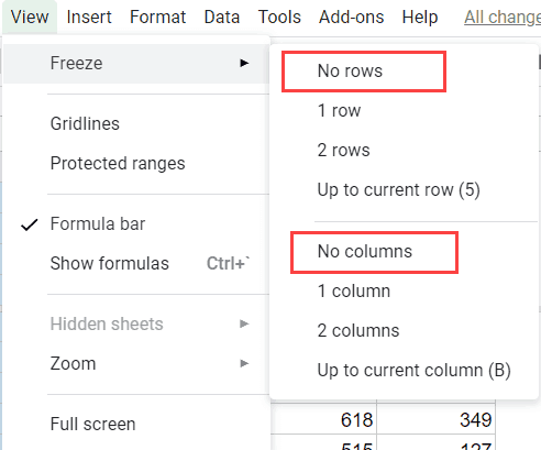
1. Click the View option in the menu
2. Hover the cursor over the Freeze option.
3. Click on No Row.
4. Again, click on the View option.
5. Hover the cursor over the Freeze option.
6. Click on No Column.

You could also use the menu keyboard shortcut: Alt +V, R, R

How to Freeze Rows on Sheets for Mobile

Here are the steps you need to follow to freeze a row or column on the Google Sheets app for Android:

1. On your main spreadsheets page, click on the spreadsheet tab name to open the options that allow you to make tweaks to your spreadsheet.
2. A small window will pop up from the bottom part of the screen. There scroll down and use the arrows to increase and decrease the number of columns and rows to freeze.
3. Click outside the window to apply the changes.

Common Issues and Troubleshooting Tips

• The primary issue you could get from trying to freeze rows or columns would be trying to freeze panes in the middle of your spreadsheet, which you cannot do. You can only freeze from the top or left-most cells. However, you can group rows and columns.
• If you have trouble freezing rows or changing frozen rows back using one method, try the other.

Frequently Asked Questions

How Do I Freeze a Specific Row in Google Sheets?

To freeze a specific row, click on it, click on View in the top bar, and then Freeze. It allows you to select the number of rows and columns you wish to freeze.

What Does It Mean to Freeze a Row in Google Sheets?

Freezing a row keeps the data of that row or column visible when your move around on your spreadsheet. This allows you to increase the readability of your spreadsheet hence making your data more valuable.

Can You Freeze Panes on Google Sheets?

To create a pane, click on the column you wish to go up to. Now, click on View and then on Freeze. There, click on Up to column X, where X is the column’s name.

How Do I Freeze the Top Two Rows in Google Sheets?

To freeze the top two rows in Google Sheets, click on View and Freeze. Click on 2 rows to freeze the top two rows in your spreadsheet.

Can You Freeze a Single Cell in Google Sheets?

While it’s not possible to freeze just one cell, you can freeze either a column or a row by highlighting it and clicking on View and Freeze.

How Do I Freeze a Row in Google Sheets Mobile?

Click on the spreadsheet name in the bottom part of the screen and then scroll down to find the freeze options. There, use the arrows to increase or decrease the number of columns and rows.

That’s it!

Now you know how to freeze a row in Google Sheets and be a lot more efficient when working with large datasets.

Fun fact: Some people also call this anchoring the cells (or anchoring the rows/columns in Google Sheets)

I hope you found this tutorial useful.