The DATEDIF function calculates age from any birth date in Google Sheets. One formula gives you the current age in years. A second version breaks it down into years, months, and days. A third option, the YEARFRAC function, handles the same job with simpler syntax.
All three are basic formulas that take a date of birth in one cell and return an age in another. Here’s how each one works.
One thing to know before you start: DATEDIF is an undocumented function in Google Sheets. It won’t appear in autocomplete when you start typing it into a cell. You have to type the full function name manually. It works, Google just doesn’t advertise it.
Counting the Number of Years
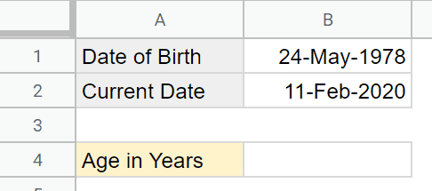
Suppose you have a birth date in cell B1 and the current date in cell B2. I’ve used the TODAY function to populate B2 with today’s date.
Two formulas calculate the current age from this data. DATEDIF is the more flexible option. YEARFRAC is simpler.
Using the DATEDIF Formula
This formula returns the total number of completed years between two dates:
=DATEDIF(B1,B2,"Y")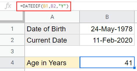
The formula takes three arguments:
| Argument | What It Does |
|---|---|
| Start Date | The birth date (the earlier date) |
| End Date | The current date (the later date) |
| Unit | Tells DATEDIF what to calculate. “Y” returns completed years. |
I used a cell reference for the current date (B2), but you can also use TODAY() directly inside the formula:
=DATEDIF(B1,TODAY(),"Y")Both return the same result. Using TODAY() means you don’t need a separate cell for the current date.
DATEDIF Unit Codes
The third argument controls what DATEDIF calculates. Here are all six options:
| Unit | What It Returns |
|---|---|
| “Y” | Total completed years between the two dates |
| “M” | Total completed months between the two dates |
| “D” | Total days between the two dates |
| “MD” | Days remaining after completed months are subtracted |
| “YM” | Months remaining after completed years are subtracted |
| “YD” | Days remaining after completed years are subtracted |
The “MD”, “YM”, and “YD” units are the ones you’ll use when building a full age breakdown (covered in the next section).
Getting Years and Months Together
If you want both years and months in a single cell, use DATEDIF twice and concatenate the results:
=DATEDIF(C3, TODAY(), "Y") & " years, " & DATEDIF(C3, TODAY(), "YM") & " months"If the birth date in C3 is March 15, 1990, and today is March 20, 2026, this returns “35 years, 0 months”.
Using the YEARFRAC Formula
YEARFRAC calculates the fraction of a year between two dates. Wrap it in INT to get a whole number:
=INT(YEARFRAC(B1,TODAY()))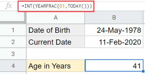
YEARFRAC returns a decimal (like 35.47), and INT strips the decimal portion so you get just the completed years. This formula is useful when you only need a year count and don’t want to deal with DATEDIF’s unit codes.
When working with dates in Google Sheets, use the DATE function if you need to enter a specific date in a formula. This prevents parse errors from dates that Google Sheets doesn’t recognize.
DATEDIF vs. YEARFRAC: When to Use Which
| Use Case | Best Formula | Why |
|---|---|---|
| Age in completed years only | Either | Both return the same result |
| Age in years, months, and days | DATEDIF | YEARFRAC can’t break down months and days separately |
| Age as a decimal (e.g., 35.47 years) | YEARFRAC | Returns fractional years natively |
| Age as of a specific date (not today) | DATEDIF | Accepts any end date, not just TODAY() |
| Simplest possible formula | YEARFRAC | Fewer arguments, no unit codes to remember |
Counting the Number of Years, Months, and Days
The formulas above return age as a single number. To get a full breakdown (years, months, and remaining days), you need DATEDIF with different unit codes in each part of the formula.
Using the DATEDIF Formula
Start with the same dataset: birth date in B1, current date in B2.
Years (total completed years between the two dates):
=DATEDIF(B1,B2,"Y")
Months (remaining months after completed years, using the “YM” unit):
=DATEDIF(B1,B2,"YM")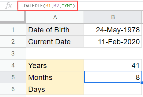
This returns 8 in this example, because 8 months have passed since the last completed year.
Days (remaining days after completed months, using the “MD” unit):
=DATEDIF(B1,B2,"MD")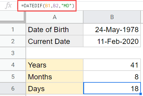
To combine all three values into a single cell, concatenate them:
=DATEDIF(B1,B2,"Y")&" Years "&DATEDIF(B1,B2,"YM")&" Months "&DATEDIF(B1,B2,"MD")&" Days"
You can replace B2 with TODAY() if you don’t want a separate cell for the current date.
Calculate Age for an Entire Column with ARRAYFORMULA
The formulas above work for a single cell. If you have a list of birth dates and need ages for all of them at once, the ARRAYFORMULA function handles that.
Suppose column A contains birth dates in cells A2 through A20. Place this formula in cell B2:
=ARRAYFORMULA(IF(LEN(A2:A20), DATEDIF(A2:A20, TODAY(), "Y"), ""))This calculates the current age in years for every birth date in the range and returns a blank for any empty cells. Without the IF(LEN()) wrapper, DATEDIF treats blank cells as the date December 30, 1899, and returns an incorrect age for every empty row.
For a full years, months, and days breakdown across the entire column:
=ARRAYFORMULA(IF(LEN(A2:A20), DATEDIF(A2:A20, TODAY(), "Y") & " years, " & DATEDIF(A2:A20, TODAY(), "YM") & " months, " & DATEDIF(A2:A20, TODAY(), "MD") & " days", ""))The ARRAYFORMULA function is one of the most useful tools in Google Sheets for applying any formula across a range. It saves you from dragging formulas down manually, and it updates automatically when new birth dates are added to the range.
Calculate Age as of a Specific Date
Sometimes you need to know someone’s age on a date other than today. An enrollment cutoff, a year-end report, or a historical reference date.
Replace TODAY() with the specific date or a cell reference containing it:
=DATEDIF(A2, DATE(2025,12,31), "Y")This returns the age as of December 31, 2025. You can also point to a cell:
=DATEDIF(A2, C1, "Y")Where C1 contains the reference date. This is useful for calculating ages at a fixed point in time, like the start of a school year or a benefits enrollment deadline.
Handling Errors with Blank or Invalid Cells
DATEDIF returns errors in two common situations: when the birth date cell is blank, and when Google Sheets doesn’t recognize the value as a date.
For blank cells, wrap the formula in an IF check:
=IF(A2="", "", DATEDIF(A2, TODAY(), "Y"))This returns an empty string instead of an error when A2 is blank.
For cells that might contain text or invalid date formats, use IFERROR:
=IFERROR(DATEDIF(A2, TODAY(), "Y"), "Invalid date")IFERROR catches any error the formula produces and returns the text you specify. You can also combine both checks:
=IF(A2="", "", IFERROR(DATEDIF(A2, TODAY(), "Y"), "Check date format"))If your dates are stored as text (a common problem with imported data), convert them first using DATEVALUE:
=DATEDIF(DATEVALUE(A2), TODAY(), "Y")The #NUM! error specifically means the start date is later than the end date. Double-check that your birth date column contains dates that are earlier than your end date.
Video Guide: Calculating Ages in a Spreadsheet
This video walks through both the DATEDIF and YEARFRAC formulas for calculating age, including the combined years/months/days version.
Wrapping Up
DATEDIF handles everything from simple year counts to full age breakdowns in years, months, and days. YEARFRAC is the faster option when you only need a whole-number age. And the ARRAYFORMULA function makes either one work across an entire column of birth dates at once.
These same formulas work for any date difference calculation, not just age. Project duration, time between milestones, days between two dates, or forecasting with future dates. Be careful when combining them with IMPORTRANGE, as that can sometimes cause errors with date formatting across sheets.
For a broader look at what’s available, the Google Sheets formulas guide covers the full range of functions.
Other Google Sheets tutorials you may find useful:
- How to Calculate Days Between Two Dates in Google Sheets
- Count Cells IF NOT Blank (Non-Empty Cells) in Google Sheets
- How to Add Time in Google Sheets
- How to Round Numbers in Google Sheets
Frequently Asked Questions
Does DATEDIF work in Google Sheets the same as in Excel?
Yes. Google Sheets supports DATEDIF with the same syntax and unit codes (“Y”, “M”, “D”, “YM”, “YD”, “MD”) used in Excel. Formulas written in one application will work in the other without modification.
Why doesn’t DATEDIF appear in Google Sheets autocomplete?
DATEDIF is an undocumented function in Google Sheets. Google hasn’t added it to the official function list or autocomplete suggestions, but it works correctly when you type the full function name. It’s a carryover from Lotus 1-2-3 compatibility that both Excel and Google Sheets still support.
How do I calculate age for an entire column at once?
Use the ARRAYFORMULA function with DATEDIF. Place this formula in the first cell of your output column: =ARRAYFORMULA(IF(LEN(A2:A20), DATEDIF(A2:A20, TODAY(), “Y”), “”)). It calculates the age for every birth date in the range and skips blank cells.
Can I calculate someone’s age on a specific date instead of today?
Yes. Replace TODAY() with a specific date or a cell reference. For example, =DATEDIF(A2, DATE(2025,12,31), “Y”) returns the age as of December 31, 2025. This is useful for enrollment cutoffs, year-end reports, or any calculation that needs a fixed reference date.
What does the #NUM! error mean in a DATEDIF formula?
The #NUM! error means the start date is later than the end date. DATEDIF requires the first argument (the birth date) to be the earlier date. Check that your dates are in the correct order and that no cells contain future dates where past dates are expected.
What is the difference between DATEDIF and YEARFRAC for age calculation?
DATEDIF returns age as whole units (years, months, or days) and lets you break age into separate components. YEARFRAC returns the fractional number of years between two dates as a decimal. Use DATEDIF when you need a detailed breakdown. Use YEARFRAC wrapped in INT when you only need a simple year count.
How do I show age as “X years, Y months” in one cell?
Concatenate two DATEDIF formulas: =DATEDIF(A2, TODAY(), “Y”) & ” years, ” & DATEDIF(A2, TODAY(), “YM”) & ” months”. The first DATEDIF returns completed years, and the second returns remaining months after those years are subtracted.
How do I handle blank birth date cells in my age formula?
Wrap the formula in an IF check: =IF(A2=””, “”, DATEDIF(A2, TODAY(), “Y”)). Without this, DATEDIF treats blank cells as December 30, 1899, and returns an incorrect result. For ARRAYFORMULA, use IF(LEN()) to filter out empty rows.