Thanks to some formulas, calculating Google Sheets days between dates has become a breeze. Using a few simple methods, you can easily calculate the number of days between two dates in Google Sheets by subtracting the dates (in case you need all the days) or using formulas to find working or non-working days.
In this tutorial, I will cover various scenarios so you can calculate Google Sheets days between dates. One thing you should know about dates is that these are just numbers that have been formatted to look like dates. Let’s get started!
Table of Contents
Calculating Total Google Sheets Days Between Dates
Suppose you have a project’s start and end dates (as shown below), and you want to quickly know the total number of Google Sheets days between dates. Since these are numbers, you can perform operations such as addition and subtraction with dates.

Since dates are numbers, you can quickly get this by subtracting the start date from the end date. The formula below will give you the total number of days between these dates.
=B2-B1
The above formula tells us that there are 274 days between the project’s start and end date.

Easy right?!
There is one thing you need to know when subtracting dates. The number of days given in the above example is exclusive of the start date. If you want to include the start date in the result, you need to add 1 to the resulting data.
To get the number of days that include the project’s start and end date, use the below formula:
=B2-B1+1
Google Sheets Days Between Dates – Workdays Only
While it’s nice and easy to get the total number of days between two dates, in most cases, you don’t need the total days but the workdays. And in this case, I assume the working days to be Monday to Friday. If the working days differ, you must change the formula (covered later in this tutorial).
After all, if it’s a work project, you can’t expect your team to work on weekends…right? Calculating the number of working days between two dates is not as straightforward as subtracting the values, but it’s not too hard (as Google Sheets has a formula for it).
Suppose you have the dataset shown below and want to calculate the number of working Google Sheets days between dates.
The formula below will give you the number of working Google Sheet days between dates:
=NETWORKDAYS(B1,B2)

The NETWORKDAYS function (as the name suggests) gives you the networking days between two dates (it takes the start and end date as the input arguments).
There are two things you need to know about the NETWORKDAYS function:
- It includes both the start and end date when calculating the number of working days
- It considers Saturday and Sunday as the weekend days. So it counts all the days that are from Monday to Friday.
While this may work well in most cases, there are two common scenarios where you may want to tweak this formula:
- You need to exclude public holidays from the working days
- Your weekends are different. For example, you may only get Sunday as the weekend, and Saturday is a working day for you. Or you are from countries where weekend days are Friday and Saturday (and not Saturday and Sunday).
The good news is — Google Sheets can handle all this easily.
Use Google Sheets to Calculate Days Between Dates For Workdays While Excluding Public Holidays
For this to work, you must list the holidays you want to exclude.
In most companies, they provide a holiday calendar that you can use. Or if you’re a freelancer or small business, you can create this yourself, too.
Below is an example of a holiday calendar that I have for 2020.

Now when calculating the number of working days between two dates in Google Sheets, I don’t want to count days that are holidays.
Thankfully, the NETWORKDAYS function already has this feature built-in. You can specify the range that has the holidays, and it will automatically ignore these while calculating the workdays.
Suppose you have a dataset as shown below:
The below formula will give you the number of working days between the start and end date while not counting the holidays:
=NETWORKDAYS(B1,B2,E2:E12)

This formula takes three arguments:
- Start Date — B1 in this example
- End Date — B2 in this example
- The range that has the holiday dates — E2:E12 in this example
Note that the NETWORKDAYS function is smart enough to adjust the holidays and weekends by itself. For example, in the below holiday dates, there are eight holidays between 1st April and 30th December.
But the NETWORKDAYS function only considers six of these, and two are on weekend days anyway (Easter and Independence Day). Since the NETWORKDAYS formula disregards weekend days when doing the calculation, it will also ensure it doesn’t remove the days twice (when it’s a weekend and a holiday).
Calculate Workdays When Weekends are Not Sat and Sun
While the NETWORKDAYS function automatically assumes weekend days to be Saturday and Sunday, this may not be the case for all.
Some of you may only have a Sunday off, and some may work in countries where Friday and Saturday are off, and Sunday is a working day.
To adjust these variations, there is another function in Google Sheets that you can use.
NETWORKDAYS.INTL — where INTL stands for international.
When you use the NETWORKDAYS.INTL function — apart from the start date, end date, and the holidays — it also allows you to specify the weekend, where the weekend could be any one day of the week or any two consecutive days of the week,
So let’s say you have the below example, and you want to calculate the number of working days when the weekend days are Friday and Saturday.
The below formula will give you the result:
=NETWORKDAYS.INTL(B1,B2,7,E2:E12)

The above formula would return 191, which is the number of days between start and end dates, with Friday and Saturday as weekend days.
This formula takes four arguments:
- Start Date — B1 in this example
- End Date — B2 in this example
- Weekend — 7 in this example. This is where you specify the weekend days you want this formula to consider. Why use 7? Check out the table below.
- The range that has the holiday dates — E2:E12 in this example
Why did I use 7 to make Friday and Saturday a Weekend Day?
This is how this formula has been coded. These numbers specify weekend days and are pre-coded in the formula.
So when I use 7, it knows that I want the weekend days to be Friday and Saturday.
Below is a table that shows all the numbers you can use and what they mean:
| Argument | Weekend Days |
| 1 | Saturday/Sunday are weekend days |
| 2 | Sunday/Monday are weekend days |
| 3 | Monday/Tuesday are weekend days |
| 4 | Tuesday/Wednesday are weekend days |
| 5 | Wednesday/Thursday are weekend days |
| 6 | Thursday/Friday are weekend days |
| 7 | Friday/Saturday are weekend days |
| 11 | Sunday is the only weekend day |
| 12 | Monday is the only weekend day |
| 13 | Tuesday is the only weekend day |
| 14 | Wednesday is the only weekend day |
| 15 | Thursday is the only weekend day |
| 16 | Friday is the only weekend day |
| 17 | Saturday is the only weekend day |
Based on the above table, if you only want Sunday to be considered as the weekend (with a six-day working week), you need to use 11 as the third argument in the NETWORKDAYS.INTL function.
Use Google Sheets to Find the Difference Between Two Dates With Workdays and Non-Consecutive Days Off
Suppose you are in a job where you only work on specific days of the week (let’s say Monday, Tuesday, and Thursday).
With such an arrangement, counting the number of working days between two given dates becomes even more challenging.
Thankfully, when the NETWORKDAYS.INTL function was being formulated; this was also taken into account.
When you’re using the NETWORKDAYS.INTL function for something such as this, you need to specify which days are working and which are not.
And you do that by using a series of seven consecutive numbers (where each number is either 1 or 0). These numbers represent the seven days of a week. The first number of the series represents a Monday. The second represents a Tuesday, and so on.
‘0’ means that it’s a working day, and ‘1’ means that it’s a non-working day. So 0000011 would mean that the first five days (Monday to Friday) are working, and Saturday and Sunday are weekends (or non-working days).
Now, you can create any combination of a week with a mix of working and non-working days. And these don’t have to be consecutive.
So in our example, where Monday, Tuesday, and Thursday are working days, the code would be 0010111.
And you can use this code in the NETWORKDAYS.INTL function as shown below:
=NETWORKDAYS.INTL(B1,B2,"0010111",E2:E12)

Note that the third argument is the string of numbers that represent working and non-working days. This needs to be within the double quotes
The last argument in this formula specifies the range that has the holiday dates.
Use Google Sheets to Calculate Date Difference For Single Weekdays Between Two Dates
Sometimes, you may not need to calculate the working days but the number of one specific weekday.
For example, suppose you want to calculate the number of Mondays that fall in a given date range (while also accounting for holidays).
A practical use of this could be when you want to know how many update calls will be done during the given dates if the call happens on Mondays.
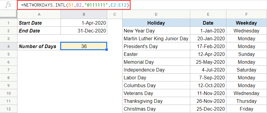
Suppose you have the data set below where you want to find the number of Mondays between the start and end date:
To calculate the number of Mondays, I will be using the NETWORKDAYS.INTL function with the string on seven consecutive numbers that represent the days in the week.
This is nothing but a variation of the example where we calculate non-consecutive working days. In this example, we need to specify only Monday as the working day; the rest are the weekend days.
So the string of numbers would be “0111111”, where 0 represents a working day for Monday.
The below formula would give you the number of working Mondays between the start and end date (while also accounting for the holidays):
=NETWORKDAYS.INTL(B1,B2,"0111111",E2:E12)
If you get the hang of how to use NETWORKDAYS and NETWORKDAYS.INTL functions in Google Sheets, you can easily manage situations where you have to calculate workdays between two days.
Use Google Sheets To Calculate Time Between Dates Using The DAYS Function
This is among the easiest ways to calculate the days between dates in Google Sheets, so long as you aren’t worried about excluding weekends, holidays, etcetera.
To use the DAYS function, you have to use this simple syntax:
=DAYS(“end_date”, “start_date”)
With this syntax, you can either type the dates manually or use cell references to populate the formula.
To use the DAYS function, simply:
- Click an empty cell
- Type =DAYS and press “Enter“
- Type the dates or click the cell references with the dates you want with a comma in between. To get the correct result, use the most recent date first
- Press “Enter“
If you’re typing the dates manually, don’t forget to use quotation marks (“”) around the dates too.


In the above examples, you can see that in cell C2 we typed the dates manually, and in C3, we used cell references and still got the same result.
Use the DATEDIF Function to Calculate the Difference Between Two Dates in Google Sheets
The DATEDIF function works similarly to the DAYS function. The main differences are that you must also provide a “Unit” for the syntax and use the start_date first instead of the end_date. So, the syntax goes as follows:
=DATEDIF(start_date,end_date,unit)
Let’s use the same data from the DAYS example:

As you can see, we had to put the older date first in this formula because you must enter the start_date first for the DATEDIF function.
We have “D” also written into our formula as our unit. This tells Google Sheets we want the results in days.
The DATEDIF function could also use the following shortcuts to show the results in different units.
- Y returns the result in years
- M is months
- MD is the difference between days while ignoring the years and months
- YM is the months in between while ignoring the years and days
- YD gives the days in between while ignoring only the years and including months
Calculate Days Between Dates in Google Sheets for a 360-Day Financial Year
If you’re working in finance, you may need to calculate days between dates for 12x 30-day periods. To do this, you can use the DAYS360 function in Google Sheets.
The syntax for this method goes as follows:
=DAYS360(start_date,end_date,[method])
With this function, you won’t have to enter the [method] if you’re working with the US version of a 360-day calendar. If you use the European method, you have to add TRUE, i.e.:
DAYS360(start_date,end_date,[TRUE])
For our example, let’s use the US version.
Unfortunately, to juxtapose the DAYS function. DAYS360 uses the start_date first, so make sure the oldest date is used first in your formula. You can also use the steps described above in DAYS to get the result you’re after.

As you can see in the example, the results read 360, so the extra 5 days of a regular calendar year are now omitted from the results.
Using the MINUS Function to Calculate Days Between Two Dates in Google Sheets
The MINUS function in Excel does not work for date calculations, but it does in Google Sheets. Technically the syntax for the MINUS function is:
=MINUS(Value1, Value2)
But, for the purposes of working with dates, you can imagine it more like this:
=MINUS(end_date, start_date)
Let’s take another look at the same data set to show how the minus function works for calculating the difference between dates. You can follow the same steps as the DAYS function but type =MINUS instead.

As you can see, you get the same results. We would still recommend using the DAYS function, though, as you get reminded of the order to enter the dates from the cues in Google Sheets. Plus, it makes your spreadsheet portable to Microsoft Excel.
Wrapping Up
Now that you can calculate Google Sheets days between dates, it should make your lives much more manageable when working out which days are working or non-working days. Hope you found this tutorial helpful!
Related: