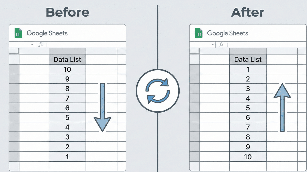
You had your data neatly in order. But now, you need to flip it. What do you do? You don’t want to rewrite your entire list manually. Let’s examine exactly how to flip data in Google Sheets, also known as Google Sheets reverse order.
Flipping a column can occur for a few reasons. You might be trying to see your data in a new way, you might need to go through it in a different order, or you might have just realized you entered it in reverse. There are actually a few ways that you can reverse order in Google Sheets. You can flip it through the Sort Range function, through sort formulas, and through indexing.
Table of Contents
Quick Answer: How to Reverse Order in Google Sheets
The fastest way to reverse order in Google Sheets is to highlight your data, navigate to Data > Sort range, and select Z to A or largest to smallest. This works instantly and requires no formulas. For data in arbitrary order, add a numbered helper column and sort by that column in descending order. For a non-destructive approach that preserves your original data, use the INDEX formula or the SORT function in a separate column.
What is Reverse Sorting and Why Would You Need it?
Reverse sorting is simply changing the order of a column or range. For example, you could change the order from alphabetical A to Z, to Z to A instead. There are plenty of reasons to do this, but the most common is for ease of reading or accessing certain data points.
In the below examples, we use elements as the subject. This makes it easy to see how sorting could become important. Sometimes you may need to have your columns in alphabetical order, but you could also need to sort by atomic number. Hopefully, you can see how this spills over into other areas of life. Product names and numbers for a store is another simple example of how this feature could be handy.
You may also have landed on this page looking for how to reverse the axis of your Google Sheet. You can do this by transposing. We cover it briefly in this article. You could also check out a full TRANSPOSE function guide instead.
Google Sheets Reverse Order: How to Flip Data in Google Sheets
In this article, we’ll begin with a list of elements (literally):

And we’re going to find a few ways to flip them.
When flipping data, keep in mind that sorting often overwrites your initial data. Save your progress before you start to change things. Luckily, Google Sheets makes it easy to revert to a previous state through version history if you make a mistake.
Now, let’s take a look at how to flip data in Google Sheets.
Related: How to Sort by Date in Google Sheets
Method 1: Flipping a Sorted Column
This is by far the easiest method of flipping a sorted column, but it doesn’t always apply.
Let’s assume that our list of elements was sorted alphabetically.

If this was the case, we could reverse the column quite easily:
- Head to Data
- Click on Sort range
- Select Sort range by column Z to A
(To flip it back, use Data > Sort range > Sort range by column A to Z.)

That was easy. Now we have the exact reverse:

This is the best method possible because it doesn’t require you to create any additional columns or enter any formulas. It’s practically automatic.
This is what we mean by “flipping” a column: putting it in the reverse order.
But your data isn’t always going to be ordered alphabetically. So, what can you do if your data is currently in arbitrary order?
Google Sheets can also reverse rows using the same method.
Related: Order Form Spreadsheet Templates
Method 2: Using a Count to Flip Your Column
Our elements are now ordered randomly:
(Just in case you’re wondering, we did this by selecting them and going to Data > Randomize Range.)

But we want them to be in the exact opposite order. Here’s what we do.
Step 1: Set up a column to the left and add numbers 1 through 8.

Step 2: Select the entire two columns and navigate to Data > Sort range.

Step 3: Sort by Column A and choose Z to A.

Optional Step 4: Everything is now appropriately flipped. Delete the helper column when you’re done.
There is an obvious issue here: what if the column is much longer? You don’t want to manually type 1, 2, 3 all the way to 1,888.

Set the second row to =A2+1 (the above row plus 1) and copy it all the way down, or use the fill handle. It will automatically update so every number equals the row above plus one. A faster option: enter 1 in your first helper cell and use =ROW()-1 in the cells below to auto-generate the full sequence without manual entry.
Method 3: Sorting the Column or Arrays Using the SORT Function
There’s another, cleaner method we can use: the SORT function. It takes a little more setup, but gives you a big advantage. Here’s how you do it in one step:
Step 1: Keep that helper column of numbers to the left. Then, in a third column, enter the following:
=SORT([data], [number_column], false)
The SORT function is told to sort column B, using column A as the sort key, in descending order (FALSE). The result appears right on the page. You end up with both the original data and the new reversed data side by side. This is a cleaner approach because it preserves your source data while displaying the reversed output separately.
Read also: Sort Horizontally in Google Sheets
Method 4: Reverse a Column Line by Line With the INDEX Function
Google Sheets can reverse columns using the INDEX function. This function works under the following syntax:
INDEX(reference, [row], [column])- reference is a range of cells to extract the data from
- row is the row number to extract data from
- column is the column number to extract data from
Here’s an example of the INDEX function reversing a column:

The formula we used is:
=INDEX($A$2:$A$8, ROWS(A2:$A$8))Notice that the only cell reference that isn’t locked with absolute values is A2. This allows the function to count down the row positions as you drag the fill handle. Each row it moves down, ROWS(A2:$A$8) decreases by one, so INDEX pulls the next item from the bottom of the list upward until the entire column is reversed.
Method 5: Reverse a Column With a Single LAMBDA Formula (Modern Method)
Google Sheets added LAMBDA and MAKEARRAY support in 2022, and this approach has become the cleanest single-cell solution for reversing a column. You don’t need a helper column and you don’t need to drag a formula down. Enter this in one cell and it outputs the entire reversed column automatically:
=MAKEARRAY(ROWS(A2:A9), 1, LAMBDA(i, j, INDEX(A2:A9, ROWS(A2:A9)-i+1)))Replace A2:A9 with your actual data range. The formula tells Google Sheets to build a new array with the same number of rows as your data, and for each row position it pulls the corresponding item from the bottom of your source range upward. The result spills into adjacent cells automatically with no extra steps.
This is the preferred method for anyone who wants a clean, formula-only solution in 2026 with no manual steps involved.
How to Reverse a Row in Google Sheets (Horizontal Flip)
Everything we’ve covered so far reverses vertical column data. But what if your data runs horizontally across a row and you need to flip it left to right?
The INDEX function handles this, but you reference columns instead of rows:
=INDEX($A$1:$H$1, 1, COLUMNS(A$1:$H$1)+COLUMN($A$1)-COLUMN())Enter this in the first cell of your output row and drag it right across the same number of columns as your source data. Each step to the right pulls the next item from the right end of your source row moving leftward.
A simpler alternative: transpose your row into a column using =TRANSPOSE(range), reverse the column using any of the methods above, then transpose the result back into a row. It takes more steps, but it’s easier to build and troubleshoot.
Flipping Multiple Columns in Google Sheets
Consider that we might have more information. In the above examples, we’re flipping only a single column. But it’s more common that we would have not only multiple rows of data, but multiple columns of data. We would want to keep that data together when sorting, or the data wouldn’t make any sense.

Now we have the element, symbol, and atomic weight. They’re all correct, but if the elements were reordered without including the other columns, they wouldn’t be.

As long as you select the entire range when you go to Sort, everything will remain in order.

You absolutely must select everything within the sorted range. If you had selected only the element column, only that column would be swapped. The symbols and atomic weights would fall out of alignment.
This is what separates Google Sheets from a relational database: there are no built-in relationships. Data isn’t automatically tied together, which means it can become disconnected when you sort only part of a range.
Transposing a Column in Google Sheets
When we say “flip” we mean to “reverse” the order of the column. But when some people say “flip” they actually mean transpose, which is something different. Here’s how to transpose data in Google Sheets:

By typing in:
=TRANSPOSE([data])You can easily switch the data from a column to a row.

You could also transpose all the data at once if you wanted to:

The TRANSPOSE function moves data from column to row and from row to column. It’s a very easy way to fix a sheet if you find that you oriented it incorrectly. And it’s something else someone might mean when they say “flip” a column.
Using Other Methods to Flip a Column
There are other ways that you can flip a column.
Realistically, if the column is short, it can be easier to just retype the entire thing. But that approach tends to introduce errors. You could forget an entry or accidentally overwrite something.
You can also use additional SORT functions and INDEX functions that are significantly more complex. They’re much more complicated and you’ll almost never need them. The methods above will handle virtually any situation you encounter.
Google Sheets Reverse Order: Frequently Asked Questions
What is the fastest way to reverse the order of a column in Google Sheets?
The fastest method uses the built-in sort tool. Highlight your data, go to Data > Sort range, and choose Z to A (for text) or largest to smallest (for numbers). This works in seconds and requires no formulas. Keep in mind that this overwrites your original order, so save a copy first if you need to preserve it.
How do I reverse a column that is in random or arbitrary order?
Add a helper column next to your data numbered 1 through N. Use =ROW()-1 to auto-fill the sequence. Then select both columns, go to Data > Sort range, sort by the helper column Z to A, and delete the helper column when done. Your original data column now appears in the opposite order.
Is there a formula to reverse a column in Google Sheets without sorting?
Yes. Use the INDEX and ROWS combination: =INDEX($A$2:$A$8, ROWS(A2:$A$8)). Copy this formula down your output column and it returns your data in reverse order while keeping the original intact. In modern Google Sheets, you can also use a MAKEARRAY formula for a single-cell solution that spills automatically.
How do I reverse a row (horizontal data) in Google Sheets?
Reversing a row uses the same INDEX logic but targets columns instead of rows: =INDEX($A$1:$H$1, 1, COLUMNS(A$1:$H$1)+COLUMN($A$1)-COLUMN()). Drag this formula right across the same number of columns as your source. An easier alternative: transpose the row into a column, reverse it using any column method, and transpose the result back into a row.
What is the difference between reversing and transposing in Google Sheets?
Reversing changes the order of items within the same orientation, so top-to-bottom becomes bottom-to-top. Transposing changes the orientation itself: rows become columns and columns become rows. Use =TRANSPOSE(range) to transpose data. The two operations are often confused but they produce completely different results.
How do I reverse the characters inside a single cell in Google Sheets?
Use this modern formula that works in current Google Sheets: =TEXTJOIN("", 1, MID(A2, SEQUENCE(LEN(A2), 1, LEN(A2), -1), 1)). Replace A2 with your target cell. SEQUENCE generates a list of character positions from the last character back to the first, MID extracts each one, and TEXTJOIN stitches them back together into a reversed string.
Will reversing my data affect other columns in my sheet?
Only if those columns fall outside your sort range. Always select the full range of related columns before sorting. Sorting only one column while leaving adjacent columns in place causes them to fall out of sync, which produces mismatched rows across your dataset.
What is the best formula to reverse a column in Google Sheets in 2026?
The MAKEARRAY approach is the most modern and efficient: =MAKEARRAY(ROWS(A2:A9), 1, LAMBDA(i, j, INDEX(A2:A9, ROWS(A2:A9)-i+1))). Replace A2:A9 with your range. It outputs the entire reversed column from a single cell with no helper column and no dragging required. This method takes full advantage of the LAMBDA functions Google added in 2022.
How to Reverse Order in Google Sheets
If you need to sort a column that’s already in ascending or descending order, the Sort range menu tool will almost always work best. For a column in arbitrary order, adding a count column lets you sort by range and then remove the helper column afterward. For a non-destructive approach that keeps your original data intact, the SORT function or INDEX formula outputs the reversed list in a separate location. And for the cleanest single-formula solution in 2026, MAKEARRAY with LAMBDA handles everything in one cell with no additional steps.
Now you know how to sort by Google Sheets in reverse order. There are many ways to flip sheets, including flipping sheets by row rather than column, and a lot of it builds on the flexible SORT function and index-based formulas Google Sheets makes available.