In most cases, data is arranged vertically (i.e., you read it from top to bottom) and there is an in-built functionality in Google Sheets to sort data that is arranged vertically.
But what if you want to sort data that is arranged horizontally, i.e, to be read from left to right (something as shown below):
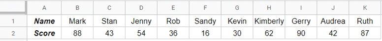
Unfortunately, there is no in-built feature in Google Sheets to sort horizontal data (i.e., sort by columns instead of rows).
But there are ways you can still do this.
In this tutorial, I will show you how to sort data horizontally in Google Sheets (using a simple formula as a paste technique).
So let’s get started!
Table of Contents
Sort Horizontally Using the SORT Function
You can use a little bit of formula wizardry to sort the data horizontally.
While the SORT function by itself would only be able to sort data that is arranged horizontally, we can combine it with the TRANSPOSE function to convert a horizontal data into a vertical one.
Suppose you have a dataset as shown below and you want to sort this data based on Student marks.
The below formula will sort the data horizontally in Google Sheets:
=TRANSPOSE(SORT(TRANSPOSE(B1:K2),2,))
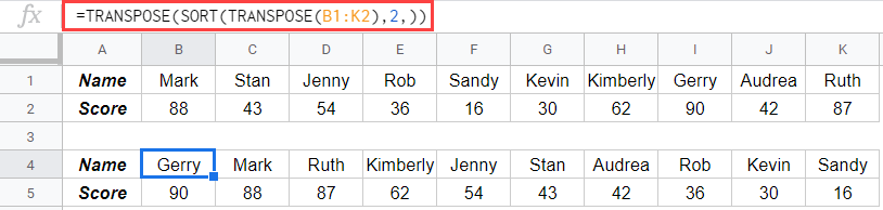
The above formula uses the TRANSPOSE function to first transpose the data from horizontal to vertical. It then uses the SORT function to sort this data based on the second row (which becomes the second column in the transposed data).
The result of the SORT function is again fed into the TRANSPOSE function to get the horizontal data back which has been sorted.
The good thing about using a formula is that it makes the resulting data dynamic.
This means that in case you change any of the values in the original data, it will automatically adjust the result to show the newly sorted data.
Some important things to keep in mind when using the formula to sort horizontally in Google Sheets:
- The result if this function is an array. You can not delete any individual cell or a range of cells in the resulting data. You will have to delete the entire resulting range at once.
- When you enter the formula and hit Enter, it will instantly fill the range of cells (which would be of the same size as that of the original data). For this formula to work, these cells where the result is expected should be empty. If any cell in this range is already filled, the formula would give an error.
Sort Horizontally By Transposing the Data Manually
If you don’t need the original data, you can also manually transpose the data, sort it (just like you sort any vertical range of cells) and then transpose it back to get the horizontal data that has been sorted.
Suppose you have a dataset as shown below and you want to sort this data based on Student marks.
Below are the steps to sort this data horizontally:
- Select the entire horizontal data that you want to sort
- Copy the data
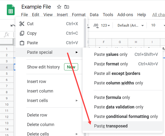
- Go to an empty cell (in the same worksheet or even on another worksheet)
- Right-click and hover the cursor over the Paste Special option.
- Click on Paste Transposed
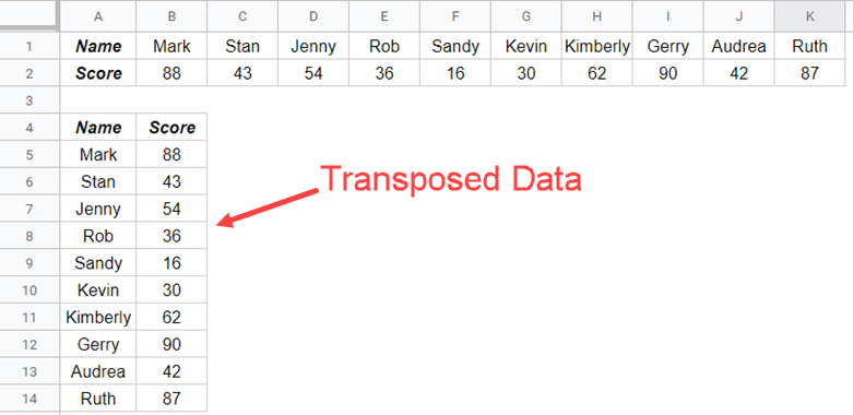
The above steps would give you the transposed data (as shown below) which you can easily sort using the in-built SORT functionality in Google Sheets.
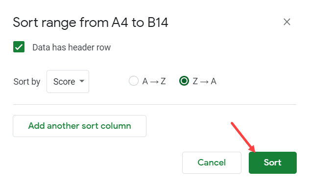
Below are the steps to sort this transposed data:
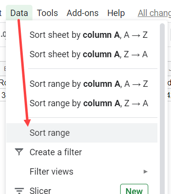
- Select the dataset
- Click the Data option in the menu
- Click on Sort Range

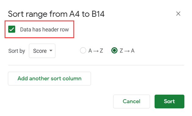
- In the Sort Range dialog box, check – ‘Data has header row’ option

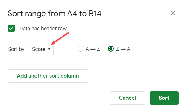
- Select ‘Score’ as the Sort by Column option
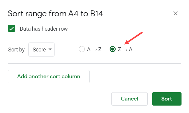
- Click on Z to A (as I want to sort this data in descending order)
- Click on Sort.
Now that you have the sorted data, you can again copy and paste it as a transposed data and it will be the same as sorting the data horizontally in Google Sheets.
So these are two ways you can use to sort data horizontally in Google Sheets.
In most cases, I would prefer using the formula method as it’s easier to use. In case you can’t use a formula, you can then use the paste transpose method to sort horizontally.
Note: If possible, try and see is you can change horizontal data to vertical. This helps in case you have to maintain and use this data as most of the formulas and functionalities in Google Sheets are made to work with a vertical dataset.
Hope you found the tutorial useful!
Other Google Sheets tutorials you may like: