Google Sheets VLOOKUP from another sheet is a simple way to pull data from other sources.
To VLOOKUP from another sheet in Google Sheets, you can use the IMPORTRANGE function with the spreadsheet’s URL and the sheet name and range. That changes the lookup range from your current sheet to a target sheet (even from another workbook).
In this guide, I’ll explain step-by-step how to use VLOOKUP Google Sheets from another sheet. Keep reading to learn more.
Table of Contents
What Is the VLOOKUP Function?
Before I show you how to use the Google Sheets VLOOKUP from a different sheet, you must first understand the VLOOKUP function.
VLOOKUP (short for Vertical Lookup) is a Google Sheets function that lets you search for a particular value within the first column of a range of cells.
Once the program finds a matching value, it looks for a value in another specified column (usually in the same row as the lookup value) and retrieves it.
The process works the same as with the Excel VLOOKUP function.
Google Sheets VLOOKUP Syntax
Before I introduce you to the process, it’s essential to understand the syntax for VLOOKUP in Google Sheets.
Below, I’ll break it down into parts, making it easier for you to understand.
The VLOOKUP Formula in Google Sheets
=VLOOKUP(search_key, range, index, [is_sorted])
Inside the VLOOKUP function, you’ll notice a few requirements. Here’s what each means:
- search_key: A search_key represents the unique identifier (or key value) you want to look up. This can be a value or a reference to a cell that contains the value.
- range: Range refers to the span of cells (in the source table) that the VLOOKUP function searches within. This range must include the search key column and the corresponding value to be retrieved. VLOOKUP always searches the first column of Range to find the search key.
- index: The Index is the column number within the range from which the corresponding value (i.e., the one in the same row as search_key) is retrieved. Therefore, the first column within the range has an index of 1, the second column has an index of 2, and so on.
- is_sorted: This is an optional parameter that can be TRUE or FALSE.
- FALSE Value: A FALSE value for is_sorted indicates the first column of Range. It doesn’t need to be sorted in ascending order. The VLOOKUP function searches for an exact match of the search_key. If there’s more than one value that is precisely equal to search_key, VLOOKUP accesses the first occurrence of the search_key.
- Note: By default, the parameter is_sorted is set to FALSE
- TRUE Value: A TRUE value means that the first column must be sorted in ascending order. The VLOOKUP function first looks for an exact match of the search_key. If an exact match is not found, VLOOKUP looks for the closest match.
The Syntax for Google Sheets VLOOKUP from Another Sheet
When you want to have Google Sheets VLOOKUP in another sheet, you’ll need to use the IMPORTRANGE function.
Remember that your IMPORTRANGE function requires a spreadsheet key and range string.
Here’s the syntax:
=IMPORTRANGE(spreadsheet_key, range_string)
- spreadsheet_key: This is the spreadsheet URL you’re importing from. It should be specified in double quotes (“ “).
- range_string: This references the range of cells you want to import. The range_string parameter should contain the sheet name and the range of cells you want.
When combining the two functions, the syntax for the VLOOKUP between two Google Sheets is as follows:
=VLOOKUP(search_key, IMPORTRANGE(“{sheetsurl}”,“{sheet name}!{cell range}”),index,is_sorted)
You’ll notice above that the sheet name and cell range in the syntax above make the range_string.
My example below shows you how to use VLOOKUP in Google Sheets from a different sheet.
How To Use Google Sheets VLOOKUP from Another Sheet
Short on time? Don’t miss my latest video on how to use Google Sheets VLOOKUP from another workbook.
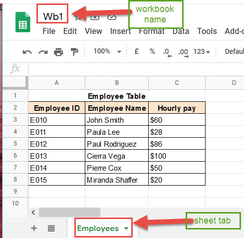
Let’s assume I have an employee table in a workbook called ‘Wb1’ (in a sheet called ‘Employees’) and a sales table in a separate workbook called ‘Wb2’ (in a sheet called ‘Sales’).
We want to access the employee’s sheet (from workbook Wb1) and then retrieve the hourly rates corresponding to employee IDs E010 and E014.
In that case, we’ll display them in cells B3 and B4 of the sales sheet (workbook Wb2).
Here are the steps you need to follow to perform Google Sheets VLOOKUP from another spreadsheet:
- You’ll need to test your IMPORTRANGE function.
- To do this, enter the IMPORTRANGE formula and add the link to your second sheet in quotation marks.
=IMPORTRANGE(“Wb1URL”,Employees!A2:C8)

- This will return the ref error. Click on it to allow access
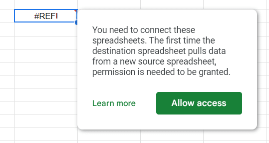
This will import the rage from your other sheet.
NOTE: You cannot allow access unless you have been granted editor access to both spreadsheets. If you only have viewer access, navigate to “File” > “Make a copy” to make a new version of the spreadsheets in your Google account.
- Click on the first cell of your target column (where you want the VLOOKUP between sheets results to appear).
- In this example, I click on cell B3 of the Sales sheet of Workbook ‘Wb1’.
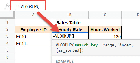
- Type =VLOOKUP, followed by opening parentheses.

- Next, select the cell containing the value you want to look up.
- For our example, select cell A3, followed by a comma.

- For our example, select cell A3, followed by a comma.

- For the second parameter, enter the function IMPORTRANGE, followed by an opening parenthesis.
- Open the workbook you want to look up (‘Wb1’ in our example) and select the sheet tab (‘Employees’).

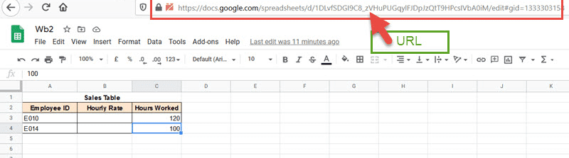
- Copy the URL of the worksheet from your browser bar.

- Return to your current workbook (‘Wb2’) and paste the URL at the end of your formula bar (remember to enclose the URL in double quotes).
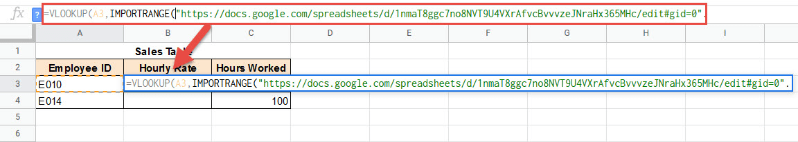
- Your formula bar should now look like this:

- Your formula bar should now look like this:
- Add a comma (,) followed by the source sheet name (“Employees” in our example).
- Add an exclamation mark (!) and type in the range of cells you want to look up from the source sheet.
- Remember to make these cell references absolute by adding dollar signs ($).
- Enclose the whole parameter (i.e., source sheet name, exclamation mark, sheet name) in double quotations.
- Add a parenthesis (to close the IMPORTRANGE function).
- Put a comma followed by the index of the column index number. This contains the values you want to retrieve.
- In our example, we want to retrieve hourly rates (the third column in the range A3:C8).
- Therefore, we’ll type the number 3.
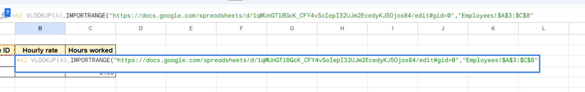
- My formula bar will show the following:

- Finally, close the parentheses for the VLOOKUP function.
- The formula bar should now show a similar formula as below:
=VLOOKUP(A3,IMPORTRANGE("https://docs.google.com/spreadsheets/d/1qMUnGT1BGcK_CFY4vSoIepI32UJm2EcedyKJ5Ojos84/edit#gid=1522021972","Employees!$A$2:$C$8"),3)
- Press the “Return” key and wait for VLOOKUP to finish processing.
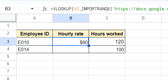
- You should now see the hourly rate corresponding to employee ID “E010” in cell B3 of your Sales sheet.

- You should now see the hourly rate corresponding to employee ID “E010” in cell B3 of your Sales sheet.
- Drag down the fill handle (located at the bottom-right corner of cell B3) to copy the formula to other cells in the column.
- You should now see the hourly rates corresponding to every employee with an ID mentioned in column A of the sales sheet.
Here is what my finished formula looks like from the above example:
=VLOOKUP(A3,IMPORTRANGE("https://docs.Google.com/spreadsheets/d/1nmaT8ggc7no8NVT9U4VXrAfvcBvvvzeJNraHx365MHc/edit#gid=0","Employees!$A$3:$C$8"),3)
How To Use Google Sheets VLOOKUP from Another Sheet: Tab
So, we talked about pulling data from another sheet. Here’s how to use VLOOKUP from another tab in Google Sheets. (Note that it’s similar to using VLOOKUP from another sheet in Excel).
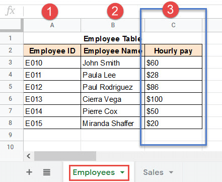
Let’s assume employee data is contained in a sheet called “Employees.”

The Sales table is in a separate sheet called “Sales.”
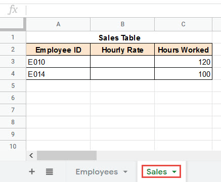
The mission: We want to access the Employees sheet and retrieve hourly rates of employee IDs “E010” and “E014.” Next, we want to display them in cells B3 and B4 of the Sales sheet.
To VLOOKUP in Google Sheets from another tab:
- Click on the first cell of your target column (where you want the VLOOKUP results to appear).
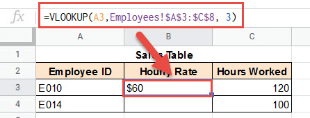
- In this example, I’d click on cell B3 of the Sales sheet.
- Type: =VLOOKUP, followed by opening parentheses.
- Select the cell containing the value you want to look up (in this example, cell A3) followed by a comma:

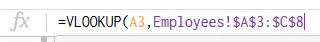
- For the second parameter, select the Employees tab (which will open the Employees sheet).
- Select the range of cells you want VLOOKUP to search (here, the cell range A3 to C8). Your formula bar should now show:

- Select the range of cells you want VLOOKUP to search (here, the cell range A3 to C8). Your formula bar should now show:

- Press the F4 key on the keyboard to lock the cell reference range.
- This ensures that these references won’t change when the formula is copied to other rows in the column.

- This ensures that these references won’t change when the formula is copied to other rows in the column.
- Enter a comma and the column index containing the values you want to retrieve.
- In our example, I want to retrieve hourly rates (the third column in the range A3:C8), so the column number is 3.

- In our example, I want to retrieve hourly rates (the third column in the range A3:C8), so the column number is 3.
- Finally, close the parentheses.
- Press the “Return” key and wait until VLOOKUP has finished processing.
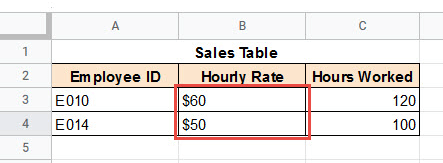
- You should now see the hourly rate corresponding to employee ID “E010” in cell B3 of the Sales sheet:

- Drag down the fill handle (located at the bottom-right corner of cell B3) to copy the formula into other cells in the column.
- You should now see hourly rates for every employee whose ID is mentioned in column A of the Sales sheet!

Related: How to Apply a Formula to an Entire Column in Google Sheets
Using Wildcards in VLOOKUP Across Google Sheets
You can use wildcard characters to expand your search in Google Sheets and find an approximate match.
As a reminder, you can use an asterisk (*) or question mark to stand in for a symbol or several characters in the text string of your search formula.
Here’s how to use wildcards:
- Asterisk (*): This symbol stands generally. Use it as any symbol and number of characters.
- Question Mark (?): This symbol represents a single character.
For example, if you typed:
- E0*, it could search partial matches such as E01, E023, and E030XY.
- E0? Would only search one extra character, like E01, E05, and E0Z.
Using Google Sheets VLOOKUP from Another Sheet: Multiple Tabs
You must have data tabs with similar structures for the following method. In the example below, I use two separate tabs containing tables containing the employee ID, hourly rate, and hours worked.
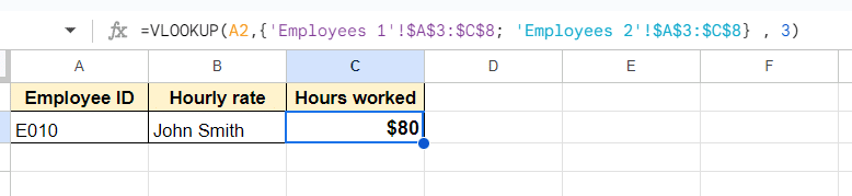
In short, If you need to VLOOKUP multiple sheets within the same workbook, you can turn the range into an array by enclosing it in curl brackets { } with semicolons between the ranges of each sheet.
Let’s break that down a bit. Using the above example, we have two tabs for employees (Employees 1 and Employees 2). You could use the following formula to search both tabs simultaneously:
=VLOOKUP(A3,{'Employees 2'!$A$3:$C$8;'Employees 1'!$A$3:$C$8},3)
This will return the results in row 3 corresponding to the value in cell A2.
Note: To avoid importing errors, you can use IF functions to pull less data from other sheets and IFFERRORs.
Tips when Using Google Sheets VLOOKUP from Another Sheets to Reference a Workbook
Here are some things you’ll want to watch for two common issues when using Google Sheets VLOOKUP different sheets.
1. Make Sure You Have Permissions
You may run into errors if you don’t have edit permissions for the workbook you’re pulling data from. Therefore, you need to ask the owner of the original spreadsheet to give you editing permissions.
Alternatively, you can make a copy of the original and then VLOOKUP the copy on your spreadsheet instead.
2. Use the Exact Range
While it may be tempting to VLOOKUP an entire row or column, this will slow the process (and make Google Sheets unusable if you do it too many times). Make sure you use the exact range to VLOOKUP.
3. Make Sure Your Ranges are Absolute
Press F4 when entering the ranges for a VLOOKUP. For example, it would change a range of C3:D14 to $C$3:$D$14.
This means the function will only search the defined cell range rather than moving the range when the formula is used for other cells.
Related: How to VLOOKUP Multiple Criteria in Google Sheets
Frequently Asked Questions
Here are the most common Google Sheets VLOOKUP from another sheet questions I hear when pulling data from anywhere besides the same spreadsheet page.
Can Google Sheets VLOOKUP from Another Sheet?
Maybe you know what to do when VLOOKUP fetches data from the same sheet. But what if the data is in a different sheet of the same workbook? Google Sheets can utilize VLOOKUP in another sheet, but there’s a slight difference in the second parameter.
Can I Do a VLOOKUP Across Multiple Google Sheets?
You can do the same thing with workbook references, like how we searched multiple criteria and tabs. Encapsulate all the ranges in squiggly brackets {} and separate them with a semicolon (;).
To add a second sheet to the above example (i.e., to VLOOKUP across multiple Sheets), it would look something like this:
=VLOOKUP(A3,{IMPORTRANGE("https://docs.Google.com/spreadsheets/d/1nmaT8ggc7no8NVT9U4VXrAfvcBvvvzeJNraHx365MHc/edit#gid=0","Employees!$A$3:$C$8") ; IMPORTRANGE("https://docs.Google.com/spreadsheets/d/1jsdjqwrqwsauhhhswuisss65shbbw/edit#gid=0","Employees!$A$3:$C$8")},3)
Can I Use the Excel XLOOKUP Function instead?
You can use XLOOKUP instead of VLOOKUP to pull data from another sheet. The syntax for the XLOOKUP function is:
=XLOOKUP(lookup_value, lookup_array, return_array, [if_not_found], [match_mode], [search_mode])
Can I use INDEX MATCH instead of VLOOKUP?
You can use one in place of the other. Specifically, you can use the index and match functions to evaluate and find a range reference. Just use this formula:
=INDEX(range, MATCH(search_key, range, [match_type]), [column_num])
Does Google Sheets have XLOOKUP?
While it wasn’t initially offered in Google Sheets, the XLOOKUP function is now a time-tested favorite. I wrote a whole guide on the subject. This was once a significant factor in using Excel vs Google Sheets. Now, the formula works for both spreadsheet tools.
Finishing up
I hope you found this tutorial helpful! Once you master this Google Sheets VLOOKUP from another sheet skill, you’ve nailed one of the most complex spreadsheet techniques. Plenty more Google Sheets functions will take your skills to the next level!
Check out some of the other guides below to jump-start your learning.