Google Sheets SUBTOTAL Function: Unbelievably Easy Guide

SUBTOTAL is a function in Google Sheets that can be incredibly versatile. With the right tips and tools, it can be dynamic and powerful, allowing you to increase your sheets’ functionality exponentially.

When using the Google Sheets SUBTOTAL function, you will find various ways to use it and multiple applications with reporting.

The 3 Primary Ways to Use the SUBTOTAL Function

1. Applying various essential functions (i.e., Sum, Count, Average) to a list of data.
2. Creating a reporting selector to view different stats from one set of data.
3. Calculating data with or without hidden rows.

This function can intimidate new or untrained users as it requires a function code to operate, but as you will see, there are ways to utilize its power without memorizing the function code list. If you’re having trouble with this, consider taking a Google Sheets course to help you learn more about this powerful program.

We’re going to show you how to do subtotals in Google Sheets using examples. Once you complete this tutorial, you will have no reason to worry about using subtotals in Google Sheets, as you will fully understand its versatility and simplicity.

Let’s get started.

Download a Copy of Our Example Spreadsheet

You can download a copy of our Example Sheet to follow along with this guide. If you find the example sheet useful, you may also want to have a look at our paid templates. You can use the code SSP to save 50% at our Gumroad store.

Google Sheets SUBTOTAL Function

Syntax

We will begin with the syntax for SUBTOTAL in Google Sheets.

The SUBTOTAL function requires two or more arguments.

1. Function Code.
2. At least one range to perform the function on.

The function codes are pictured below and are available in Google Sheets at any time. To do this, you will first need to begin typing the function =SUBTOTAL.

Then, in the formula help section at the bottom left, you will see a “Learn More” button. Select that.

Please Note: If the formula help section is not visible, there will be a blue question mark box; click that or push F1 to open the formula help section.

Function Code

Once you have selected the Learn More button, a right-hand sidebar will appear; in this you will see a detailed explanation of each function code. This may come in handy if you forget.

The Google Sheets subtotal function codes are as follows:

• 1 = AVERAGE
• 2 = COUNT
• 3 = COUNTA
• 4 = MAX
• 5 = MIN
• 6 = PRODUCT
• 7 = STDEV (Standard Deviation)
• 8 = STDEVP (Standard Deviation Population)
• 9 = SUM
• 10 = VAR (Variance)
• 11 = VARP (Variance Population)

As you can see, there are 11 functions built into the SUBTOTAL function in Google Sheets. Additionally, you can tell the function to ignore hidden cells by changing the function code. You use the same code, but you make it in the 100s. To run the functions while ignoring the hidden cells, one would use the below codes:

• 101 = AVERAGE
• 102 = COUNT
• 103 = COUNTA
• 104 = MAX
• 105 = MIN
• 106 = PRODUCT
• 107 = STDEV
• 108 = STDEVP
• 109 = SUM
• 110 = VAR
• 111 = VARP

Here is an example of the SUBTOTAL formula being used to sum a range of data. As you will notice, the function code of 9 communicates that it should sum the range.  

=SUBTOTAL(9,A1:A10)

How to SUBTOTAL in Google Sheets

One may ask why you would use the SUBTOTAL function in Google Sheets to run a SUM function? Wouldn’t it be more simple to use the SUM function? These questions are completely understandable and logical. However, situations exist that would make the SUBTOTAL function more valuable and effective. One such situation is how to add subtotals in Google Sheets.

Suppose you had the following dataset and you chose to use the SUM function in place of the SUBTOTAL function:

In the chart below, you will see that the SUM function is in each total cell and the grand total cell at the bottom of the table.

If you were to manually add up all of the totals, you would find that the Sum of the Average Projected Sales and Actual Sales does not match the totals listed. However, each Quarter Total is correct. Because the SUM function is adding all the numbers in the set range. As a result, the Quarterly totals are being added into the figures making this method ineffective and problematic.

To avoid that, we need to change all of the SUM functions to SUBTOTAL functions. The SUBTOTAL function does not add in the other subtotal functions; thus, you get the correct totals. The example below shows how to create subtotals in Google Sheets:

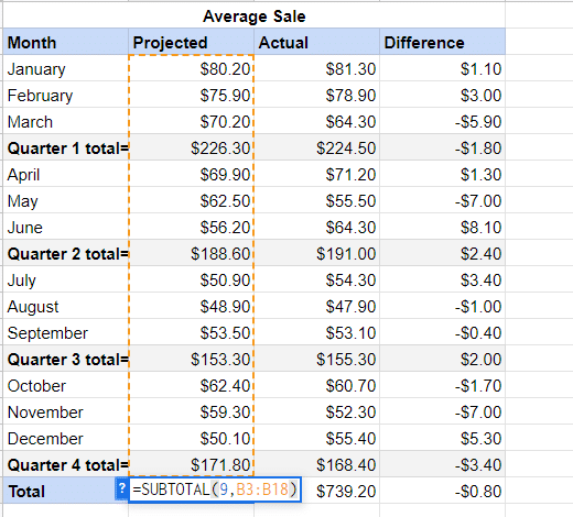
Google Sheets SUBTOTAL Function for Filtered or Hidden Data

Suppose we have a large data set that is categorized and set up to filter by month. We have total cells to review our reports data. The goal is for the Total Cells to adjust based on the filter. So if we are looking at January’s data, the total cells need to reflect that.

Also, if we hide a row, we want the data cells to reflect that as well. The first thing to note is that, as you will see in the example, when the SUM function is used, it does not adjust when the data is filtered or hidden. With the SUBTOTAL function, the opposite is true.

You will see the total in question at the bottom of the sheet remainis the same even though some months are hidden.

Initially, everything appears the same with the exact results. However, if we filter the results by month and get the Google Sheets subtotal filter, we will begin seeing the differences.

To do this,

Step 1: select the green filter drop-down at the top of the Month column.

Step 2: Select the month in question and hit OK. You will now see that the data has changed, and many rows are filtered.

Step 3: Type the subtotal formula in the cell for total.

You will also notice that the SUM cells in the table below are unchanged. However, the Filtered cells that use the subtotal function are adjusted only to show unfiltered cells.

Additionally, if there is an outlier or row of data you would like to exclude, you can hide that row of data, and the SUBTOTAL function that removes hidden rows is now updated even further.

How to Use the SUBTOTAL Function to Create a Dynamic Report Function Selector

The most versatile method of using the SUBTOTAL function on Google Sheets is to create a Report function selector. Allowing you to change the metrics being seen in the report quickly and can be done by combining various functions and operations with the SUBTOTAL function. To do this you’ll need to use the Google Sheets subtotal with conditions.

In our example sheet, we can create a dynamic report  that will return information on various things like average, sum, max and min for the Actual sale column.

 It is relatively simple and the steps are below.

The first step in this is to create a function table for the SUBTOTAL functions available.

We’ll use this list for a Data Validation (Drop-Down) and a VLOOKUP function in the following steps.

We’ll create a data validation that refers to this list in the cell you wish to make your selector drop-down. To do this:

Step 1: Create a list for the drop-down menu. Right-click the cell.

Step 2: Go to Data >Data Validation.

Step 3: Click Add rule.

Step 4: Under criteria, choose Dropdown (from a range)

Step 4: Select the aggregation column range from the list we created in step 1 and click OK.

Now that you have created the data validation drop down, you should see an arrow on the cell that lets you double click and select your option.

The remaining steps are all related to writing the functions to get the results we need.

Step 5: We will be nesting a VLOOKUP function within our SUBTOTAL function. Nesting is when you use multiple functions together to get the desired result. To do this, you will write the following in the cell.

=SUBTOTAL(VLOOKUP(G2,J1:K9,2,FALSE),D:D)

• The VLOOKUP is looking at the table we created in step 1, in the range AH4:AI14. It is looking for the contents in the drop-down cell we created in E54. Once it finds the correct row, it looks to the second column of the range for the result. It then plugs that number into the SUBTOTAL function for the function code.

Step 6: Now create a cell for the Ignore Hidden Rows function and input the below. It is the same as above, except we added “100+” to the Vlookup section, which will cause it to use the ignore hidden cells function code.

=SUBTOTAL(100+VLOOKUP(G2,J1:K9,2,FALSE),D:D)

• Your selector is now functional and ready to use. However, if you want to make it more advanced, you can create a checkbox to control the ignore hidden cells function.

• Then in the results cell, you will need to enter the below function. You are using the same functions as above but controlled by an IF statement that will look at the check box and then decide which results to show. Allowing the user to toggle between show or ignore these cells.

=SUBTOTAL(IF(H3=TRUE,100+VLOOKUP(G2,J1:K9,2,FALSE),VLOOKUP(G2,J1:K9,2,FALSE)),D:D)

Frequently Asked Questions

Why Use SUBTOTAL Instead of SUM?

Unlike the SUM function, SUBTOTAL can be used repeatedly in the same column to add a Google Sheets subtotal by category without affecting the calculation. It can also be used when filtering data to exclude some values from the calculations, while the SUM function will calculate all the values whether they are filtered out or not.

Is SUBTOTAL the Same as Total?

A subtotal is the total of a specific set of data in a range while total means the sum of all the data in the range. The SUBTOTAL Google Sheets function can be used to accurately find the sum of subsets in the data as well as the whole data at the same time.

Conclusion

Google Sheets has many beneficial functions. One of these is the SUBTOTAL Function. It has a highly dynamic nature and can benefit any reporting system on Google Sheets. Hopefully this tutorial has shown you how to SUBTOTAL in Google Sheets.

You can also check out our guide for how to add a calculated field in Google Sheets.

Related:

• How to Multiply in Google Sheets (Numbers, Cells or Columns)
• Easy Guide: How to Subtotal in Google Sheets
• How to Divide in Google Sheets (Numbers, Cells, or Columns)
• How to Merge Cells In Google Sheets
• How to Apply a Formula to an Entire Column in Google Sheets
• Slow Google Sheets? Easy Ways to Speed Up
• How to Compare Two Columns in Google Sheets
• How to Use SUMIF function in Google Sheets? Examples!