How to Hide Zero Values in Google Sheets (2 Easy Methods)

Do you need to hide zero values in Google Sheets? You’re in the right place. Sometimes, your data set looks cluttered with a bunch of zero values. That might be fine for backend data, but for a presentation, you might prefer to hide zero values in Google Sheets to make it readable.

That’s where I come in. In this tutorial, I’ll show you the best methods you can use to hide zero values in Google Sheets. I will also cover a method you can use to remove them completely. Read on for my step-by-step guide.

Method 1: Hide Zero Values using Custom Formatting (Best Method)

I am putting this method first because it is the most robust way to handle zeros. While conditional formatting (Method 2) works well, it only “paints” over the zero. To truly hide zero values while keeping the data intact for formulas, use the custom formatting method.

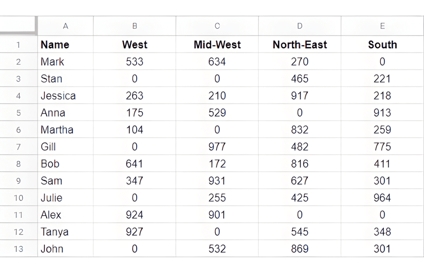
Let’s use the dataset in the screenshot below. Here, we want to hide zero values in the spreadsheet. To do this, we’ll use a specific custom formatting instruction in Google Sheets.

Follow along to hide those pesky zero results in your worksheet:

1. Select the entire dataset (A1:E13 in this example).
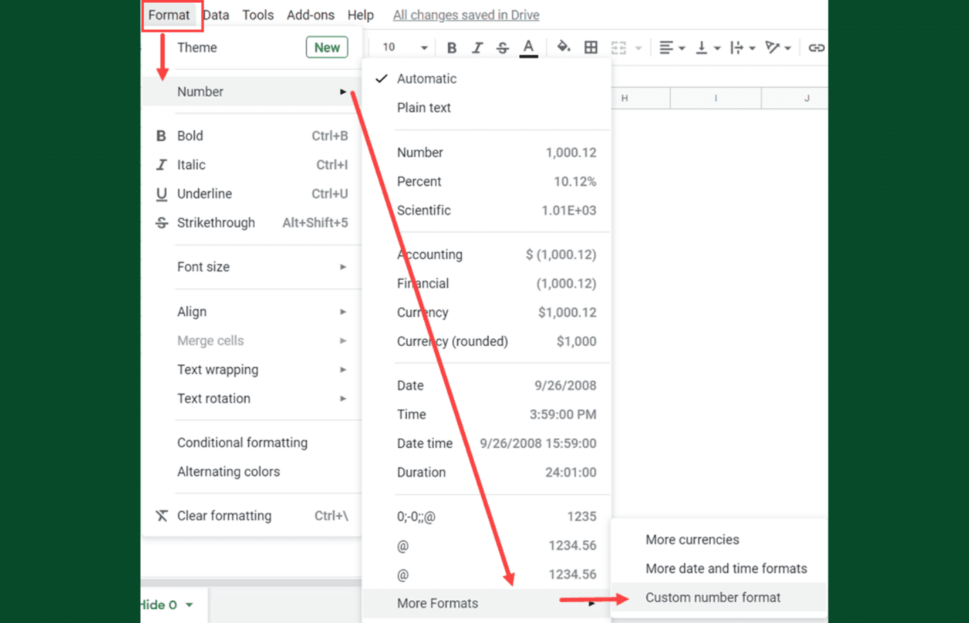
2. Click the Format option in the menu.
3. In the options that appear, go to Number > Custom number format. This will open the Custom Number Formats dialogue box.
   
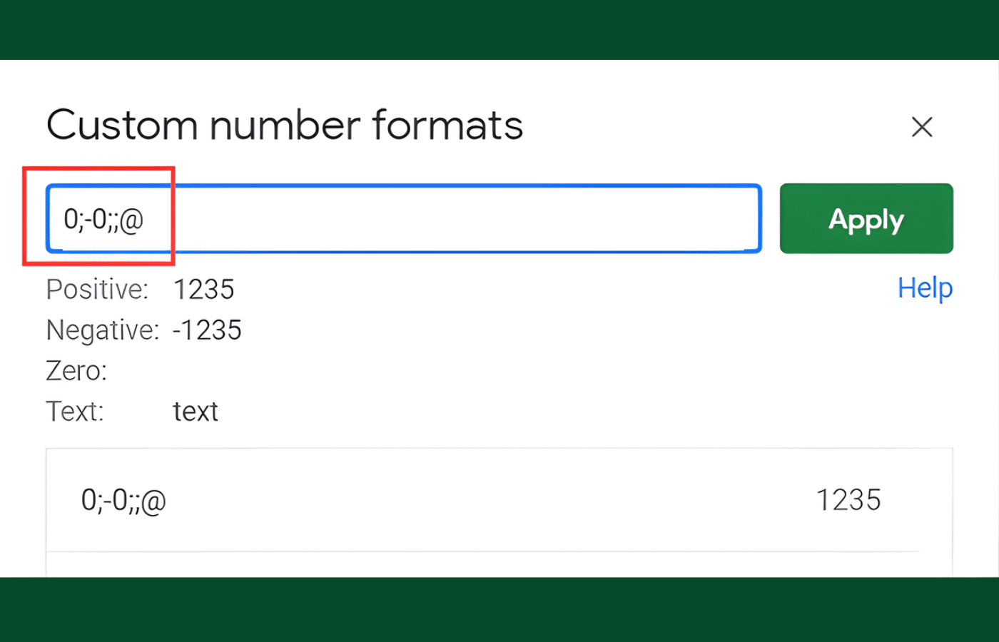
4. In the Custom number formats dialogue box, enter the following format: 0;-0;;@
   
5. Click on the Apply button.

As soon as you click Apply, the zero values are hidden. All other cells remain unchanged. Let’s talk about why that happens.

Custom Formatting Explained

In that dialogue box, you copied and pasted my 0;-0;;@ format. It might look like a confusing jumble, but it helps to break out the syntax to understand what it means. Note that this also helps you with formatting positive and negative numbers, if you’re interested.

The custom format syntax in Google Sheets is divided into four parts:

Positive Numbers; Negative Numbers; Zeros; Text

For each of these formats, you can specify how you want the cell to display the value. In this example, I have specified the following:

• Positive Numbers: These should look as is and is specified by using the 0.
• Negative Numbers: These should be displayed with a negative sign at the beginning, specified by -0.
• Zeroes: These should be hidden as we have left the format empty (note the double semi-colon ;; with nothing between them).
• Text: Show the text as is and is specified by using the @ symbol.

Look familiar? In the above syntax, you’ll notice that we have a 0 digit in the positive number location, another 0 in the negative number location, and we’ve left the zeroes location blank. That means that it’s entirely hidden in our worksheet.

Important Note: When you hide a zero value in a cell using this method, it only hides the display of the value. This means that while the cell may look as if it’s empty, the 0 value is still in the cell. In case you use these cells for any calculation, these zero values will be used.

Method 2: Hiding Zero Values with Conditional Formatting

You don’t need to delete every zero value to hide it in Google Sheets. Instead, you can use conditional formatting. This method essentially “masks” the zero by making the font color match the background color (usually white).

Below, I’ll show you how to automatically check whether a cell has a zero value and then apply conditional formatting to those cells.

Suppose you have the same dataset as shown above and you still want to hide all the zero values. There’s another way using conditional formatting.

Below are the steps to use conditional formatting to change the font color and hide these zero values:

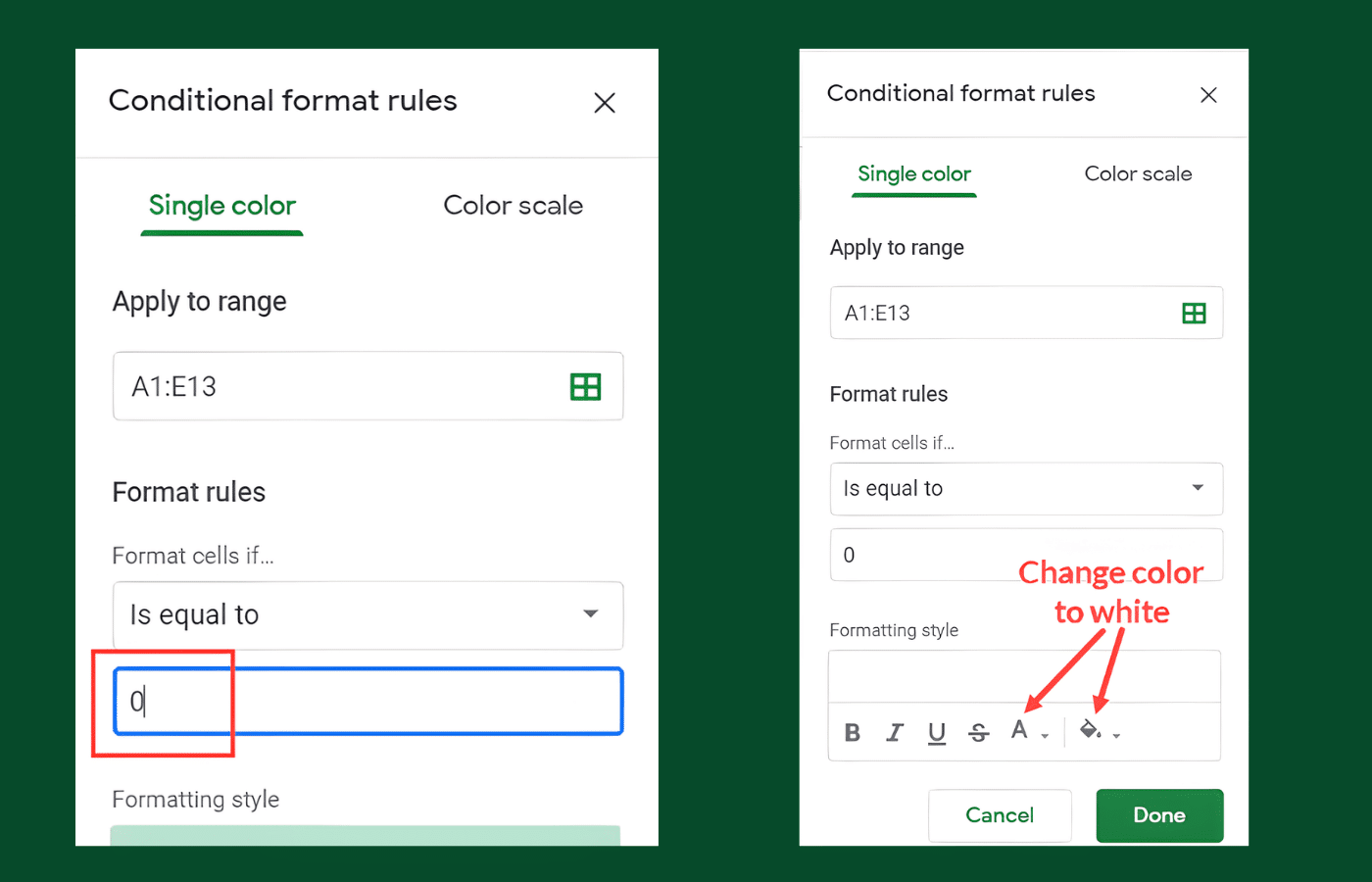
1. Select the entire dataset (A1:E13 in this example).
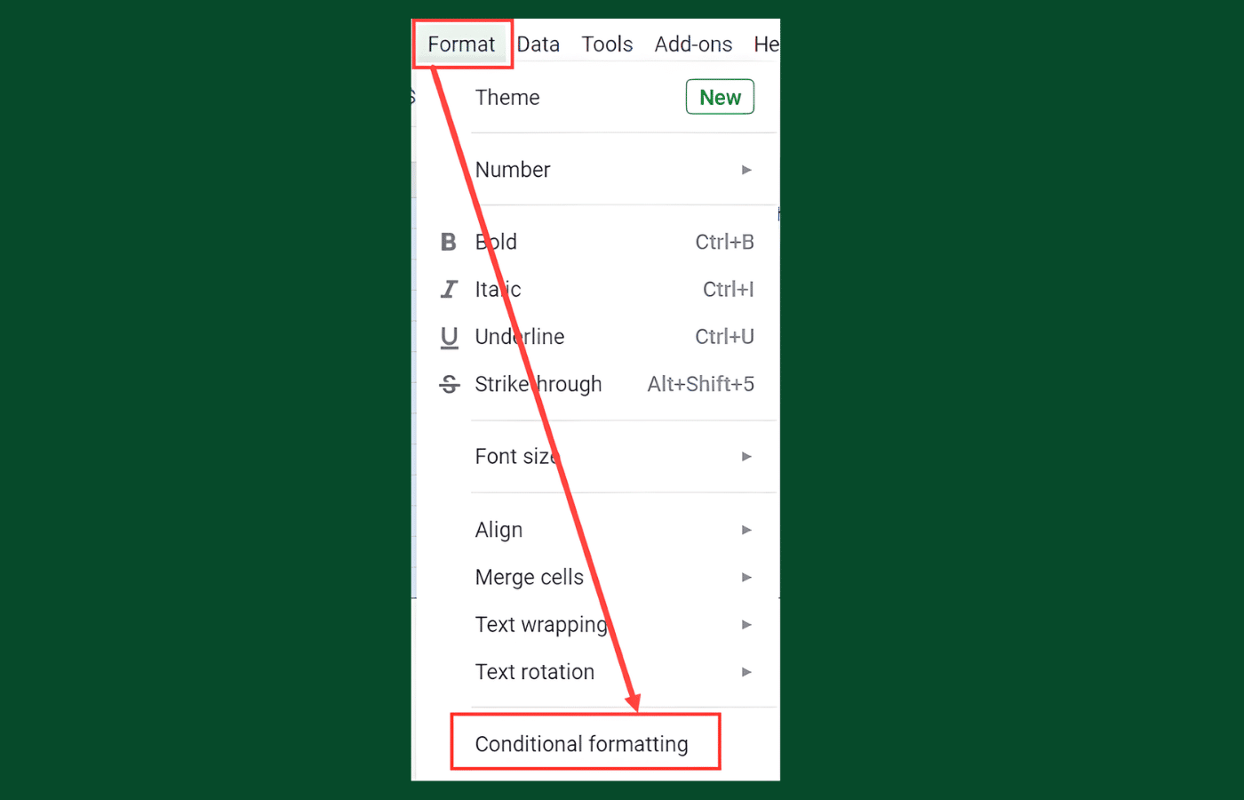
2. Click the Format option in the menu.
3. Click on Conditional Formatting. This will also open the Conditional Formatting pane in the right side of the worksheet.
   
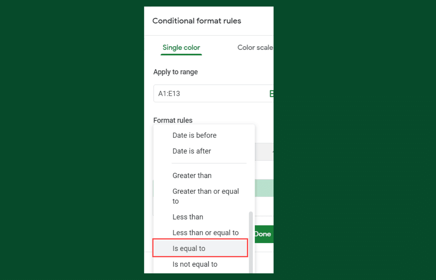
4. In the ‘Conditional Formatting Rules’ pane, click on the ‘Format cells if’ drop-down.
5. Click on ‘Is equal to’ option (you may have to scroll a bit to see this option in the list).
   
6. In the field below the ‘Is equal to’ selection, enter 0.
7. In the Formatting style options, change the font color (and cell fill color if needed) to white.
   
8. Click on Done.

The above steps would hide all the zero values and the cells would appear blank.

Remember, the cells just look blank, but these are not blank. These cells still have the zero values (as we have not removed the zero values, only changed the color to make the cells look blank).

Method 3: Return a Blank Cell Using the IF Function

Looking for even more ways to change the look of your spreadsheet? Consider using the IF function as an alternative to hiding zeros in Google Sheets.

The previous two methods are great if you already have data. But what if you are building a calculator and you want the result to be blank instead of 0? You can use a formula for that.

The Formula:

=IF(A1-B1=0, "", A1-B1)

In this example, if A1 minus B1 equals 0, Google Sheets puts an “empty string” ("") in the cell. Otherwise, it performs the math. This is very popular for financial dashboards where you only want to see variance if it actually exists.

Method 4: Find and Remove Zero Values (Destructive Method)

The above methods will hide the zero values in Google Sheets, but the value would still be in the cells. That’s helpful when you just want the data to look cleaner during review. But what if you want to remove zero values entirely?

There’s a quick solution to that too. In case you want to remove the zero values (so that the cells are empty), use the steps covered below.

First, suppose you have a dataset like the one in my screenshot below and want to remove all the zero values in the same dataset again.

Below are the steps that will find all the cells with the zero values and then remove these:

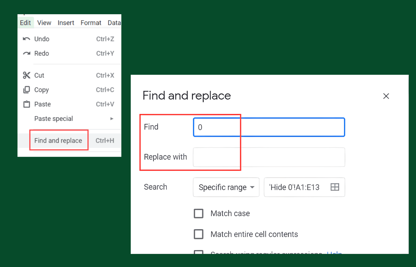
1. Select the entire dataset (A1:E13 in this example).
2. Click the Edit option in the menu.
3. Click on Find and Replace option. This will open the Find and Replace dialog box (you can also use the keyboard shortcut Control + H).
4. In the Find and Replace dialog box, enter 0 in the ‘Find’ field and leave the ‘Replace with’ field empty.
   
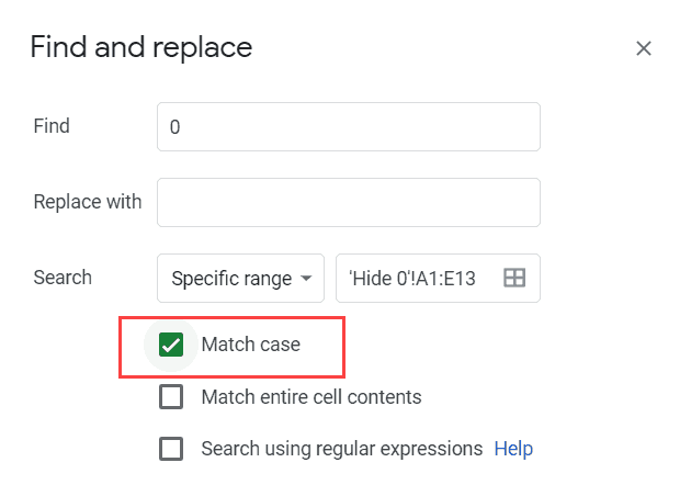
5. Important: Check the option, ‘Match entire cell contents’. If you don’t do this, you might accidentally delete the zero from numbers like “10” or “2024”.
   
6. Click on Replace All.
7. Click on Done.

The above steps would replace all the cells that have zero values with blanks. If you’re looking for a deeper dive, I cover it in much more detail in my article on the Find and Replace function in Google Sheets. That’s the best way to completely remove null values from your spreadsheet.

Related Reading: How to Install ChatGPT in Google Sheets.

Frequently Asked Questions

Sometimes, readers ask for my expertise with follow-up questions on my guides. That’s why I made this Q&A. Here are some of the most common questions I hear about hiding values in Google Sheets. If you have any other questions, please let me know in the comments!

How do I highlight all the zeros in my spreadsheet?

If you want to highlight duplicates in your spreadsheet, you’ll use conditional formatting. It’s the same process I outlined in Method 2 above, but instead of choosing white text, you’ll choose a bright highlight color (like yellow or red) to make the zeros stand out.

How do you hide zero values in Excel?

Microsoft Excel has a native setting for this. In the Excel Options (Advanced > Display Options for this Worksheet), there is a simple checkbox that says “Show a zero in cells that have a zero value”. Google Sheets does not have this specific checkbox yet, so we use the Custom Formatting methods described above.

Is it better to hide or remove zero values?

It’s usually better to hide zero values (Method 1) than to remove them entirely. Generally, you want to protect as much of your data as possible. If you remove the zero, the cell becomes “Blank” or “Null,” which can break future formulas that expect a number.

Can I show a dash instead of a zero in Google Sheets?

Yes, some people prefer to use dashes for zero values (this is common in accounting). You can do that with the custom format method. Instead of 0;-0;;@ you would use 0;-0;-;@. You could also show an asterisk in place of a zero, or you could have it display the term “null” instead.

Can I hide zeros in a specific range or array?

Yes, you can use any of the methods above to hide zero values in a specific range. Just make sure only that range is selected when you apply your formatting. If you have a whole column of zero values, just hide the whole column.

Conclusion

I hope this helped you hide zero values in your Google spreadsheet. As always, I’m here to help if you need me! Like my commentary on spreadsheets and formulas? Sign up for my newsletter below, or check out the YouTube channel for more spreadsheet advice.

You may also like the following Google Sheets tutorials:

• How to Hide Gridlines in Google Sheets
• How to Color Alternate Rows In Google Sheets
• How to Transpose Data in Google Sheets
• How to Show Negative Numbers in Red in Google Sheets

This article was checked by Jim Markus.