Functions are the engine inside the cells of your spreadsheet. They power most of the work you do in Google Sheets and Excel, from basic arithmetic to forecasting and data cleanup. Whether you’re calculating compound interest, concatenating cells, or projecting financial expectations, you’ll end up using formulas. If you already know the function you want, use the site search. If you want quick answers and a clear path forward, start below.

• Quick answers to common formula questions
• Simple formulas vs complex formulas
• Popular formulas in Google Sheets
• Understanding syntax
• Spreadsheet formula examples
• Filtering and extracting subsets of data
• Text cleanup and transformations
• Reshaping data with TRANSPOSE
• Troubleshooting common formula errors
• Spreadsheet formula cheat sheet

Quick answers to common formula questions

How do I start a formula in Google Sheets?

Use the equal sign to automatically start a formula. Autocorrect makes this super easy.

What is the formula to add up a column of numbers?

The SUM formula is the easiest way to do this. We have a guide on how to quickly sum a column, too.

How do I subtract one cell from another in Sheets?

The minus sign is the easiest way to subtract in Google Sheets. But there’s so much more you can do with it. We like using the subtract formula in arrays, across multiple worksheets, and even with dates and times. See our guide on how to subtract in Google Sheets.

How can I multiply two numbers in Google Sheets?

You can use the * on your keyboard to multiply numeric values in your spreadsheet. You can also use the MULTIPLY function. Here’s a practical guide to multiply in Google Sheets.

How do I use VLOOKUP in Google Sheets?

VLOOKUP stands for vertical lookup, and it helps you find specific information in a large range of cells. You can do case-sensitive lookups with it, and you can also use it compare data sets. Full walkthrough: VLOOKUP.

How do I write an IF statement in Google Sheets?

The IF formula helps you create conditions for calculations in your spreadsheet. The simplest is IF THEN calculations. But you can also do IF CONTAINS and IF NOT. You can even write multiple conditions with the IFS formula. See: IFS formula.

How can I highlight duplicates using a formula?

There’s an easy way to highlight duplicates in Google Sheets. The key is using conditional formatting and the COUNTIF function, as Sumit shows in the guide here at Spreadsheet Point: highlight duplicates in Google Sheets.

How do I copy a formula down the whole column?

To copy a formula and have it automatically update, you can click and drag on the bottom right corner of the cell. The spreadsheet guesses what you want, and it can make mistakes. Use dollar signs to tell the sheet you don’t want to change specific parts of your formula.

Is there a formula to count how many cells have text in them?

You can count cells with text in Google Sheets with either the COUNTA or COUNTIF functions. They’re both helpful. The guide at Spreadsheet Point also shows how to count cells with a wildcard or with the SUMPRODUCT function. Sumit’s guide also covers counting names, cells that contain part of a string, and cells that don’t contain specific text. See: count cells with text in Google Sheets.

How do I calculate the average of a specific range?

The AVERAGE function calculates the average for a range of numeric values. To use it, type =AVERAGE( and then select the range you want to calculate.

How can I combine the First Name and Last Name columns into one?

There are several ways to combine the values in two columns into a single cell. We like to use the ampersand symbol for simple combinations. Drop it in a formula between the cells you want to combine, and it combines them for you. As an example, if you have “Spreadsheet” in cell B1 and “Point” in cell C1, use =B1&C1. More options here: combine cells.

How do I pull data from one Google Sheet to another?

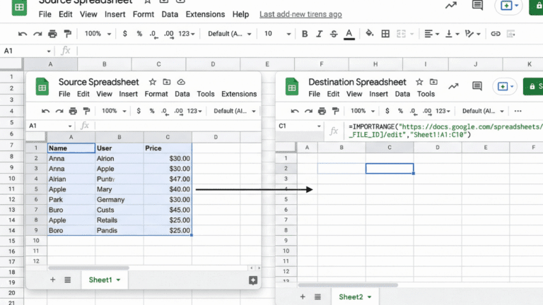
To make a formula that references another sheet, use the IMPORTRANGE function with your target URL in quotes. It looks like this, =IMPORTRANGE(“URL”). And those quotes are vital. You’ll get an error if they’re not included. See: reference another sheet.

How do I calculate the number of days between two dates?

To calculate days between dates, use a simple subtraction formula. The dates are stored as numeric values in Google Sheets, so this is usually the easiest approach. For more advanced calculations, you can also use the DAYS or NETWORKDAYS functions. Guide: days between dates.

How do I insert today’s date automatically?

The TODAY function gives you today’s date. Drop it into any cell and the spreadsheet automatically updates.

How do I sum numbers based on a specific condition (SUMIF)?

The SUMIF function returns the sum of a range of cells that match a specific condition, also called a criterion. We use this to get conditional sums based on date conditions, logical operators, and wildcard values. Guide: SUMIF.

Why am I getting a “Formula Parse Error” in Sheets?

A parse error in Google Sheets is a blanket term for a formula error. It usually means something in the syntax is off, like a missing parenthesis, a misplaced comma, or an invalid range reference. For example, #REF! means the reference does not exist in Google Sheets, so you should check that the range in the formula points to an appropriate part of the spreadsheet. Full guide: parse error.

What does the dollar sign mean in a Google Sheets formula?

This is one of the most powerful features for formulas. Add a dollar sign when you do not want Google Sheets to change that specific part of your formula when you fill or drag it across a range of cells. This is something we use constantly.

What is the difference between VLOOKUP and XLOOKUP?

The XLOOKUP Google Sheets function is a more recent addition and helps Google catch up to Microsoft’s superior search functions. It’s more powerful than VLOOKUP, and it can work with a table or range instead of only a vertical layout. Guide: XLOOKUP.

How do I use the QUERY function in Google Sheets?

The QUERY Google Sheets function helps you apply a query to a data table within Google Sheets. I often use it to extract subsets of data from main datasets, which makes analysis faster. Guide: QUERY.

Is there a formula to calculate someone’s age from their birthday?

Just subtract your birthday from today in a cell. Assuming you have your birthdate in cell A1, you can use =(TODAY()-A1)/365 to estimate your age in years.

How can I round numbers up or down using a formula?

You do not always need a formula to round. You can use the quick menu at the top of the sheet. For rounding inside calculations, functions like ROUND, ROUNDUP, and ROUNDDOWN are helpful.

How do I get rid of the #DIV/0! error?

If you’re seeing #DIV/0!, it means your formula is trying to divide by zero. Check your reference cells and make sure none are empty, and consider wrapping the calculation in IFERROR if you want to show a blank instead.

How do I name a range of cells to use in a formula?

Select the cells you want, then go to Data, Named ranges, and enter a name. After that, you can use the name in formulas like =SUM(Profits) or =VLOOKUP(A2, RevenueTable, 2, FALSE) instead of typing cell references.

Can I translate languages using a Google Sheets formula?

Yes. You can use GOOGLETRANSLATE, for example =GOOGLETRANSLATE(A1,”en”,”es”) to translate English in A1 into Spanish. If you do not know the source language, use “auto” as the second argument.

How do I import live stock prices into Google Sheets?

The GOOGLEFINANCE function pulls finance information into your spreadsheet automatically. It’s something we use in our stock tracker and investment tracking spreadsheets.

How do I use ArrayFormulas to apply a formula to a whole row?

Wrap your logic in ARRAYFORMULA and switch single-cell references into a row range. For example: =ARRAYFORMULA(IF(LEN(B2:Z2), B2:Z2*2, )). This applies the calculation across the whole row segment and keeps blanks blank instead of returning zeros.

Simple formulas vs complex formulas

Most people start with simple formulas: adding, subtracting, and basic multiplication across numeric values. These include the SUM function. They’re usually a single operation applied to one or two cells and result in a specific value. Complex formulas typically combine multiple functions, logic, and cell ranges. A complex formula might include a logical_expression inside IF, nested functions, a criterion for FILTER or SUMIF, or an array formula that returns multiple values at once. The good news is that the building blocks do not change. You still start with =, then layer functions in a way that reads like a sentence.

Popular formulas in Google Sheets

Many people start with finance use cases. A common example is using a spreadsheet to calculate compound interest, then adapting those patterns to project long-term growth. We also use spreadsheet formulas for linear regression, which is helpful for trendlines, forecasting, and quick what-if analysis. And plenty of formulas are universal across categories. You might need to concatenate cells any time you’re cleaning imported data or building a quick report.

Understanding syntax

We cover the syntax of Google Sheets and Excel functions in every one of our articles. Any formula starts with an equals sign, then the function name, then arguments inside parentheses. For example:

=REGEXMATCH(text, expression)

The first term is the name of the function. The terms in parentheses are arguments. Those vary by function, so we give examples for exactly what you need. A few syntax terms you will see often:

• logical_expression: a test that returns TRUE or FALSE, for example A2>=10
• criterion: a condition used to match values, for example “>=1/1/2026” or “*West*”
• numeric values: numbers or date values that Sheets can calculate with
• char: a character inside text, like a comma, dash, or space

Spreadsheet formula examples

We include step-by-step instructions on how to use each formula, for Google Sheets and Excel functions. Read my guide to ISERROR, for example. I give a complete walkthrough on how to use it to highlight rows with errors, including how to expand the pattern across multiple rows or an entire sheet. Two other examples many people need early on:

• Maximum value: use MAX(range) to return the maximum value in a provided source range
• Minimum value: use MIN(range) to return the minimum value in a range
• Mode: use MODE(range) to return the most common numeric value in a range

Filtering and extracting subsets of data

Filtering is one of the fastest ways to extract a subset of rows that match your logic. The FILTER function uses a criterion or logical_expression to return only the matching rows. When you need database-style extraction, sorting, and grouping, the QUERY function is often a better fit because you can express more complex logic across a table.

Text cleanup and transformations

Text work is where spreadsheets quietly become powerful. You can merge values, remove unwanted characters, and standardize formatting across messy imports. Two functions you will see constantly:

• SUBSTITUTE: replace a specific char or substring inside text
• CONCATENATE or &: combine strings, names, and labels into a single output

Reshaping data with TRANSPOSE

TRANSPOSE flips the orientation of your data. It turns rows into columns and columns into rows, which is useful when you inherit a dataset in the wrong shape for analysis or charting.

Troubleshooting common formula errors

If your formula breaks, start by identifying the error message. Most issues come down to references that do not exist, mismatched syntax, or missing matches in lookups.

How do I fix the #N/A error in my VLOOKUP?

We see #N/A with VLOOKUP when there’s no match found. Double-check the lookup value, confirm you’re referencing the correct range, and confirm you’re using the right match type in the final argument.

Why am I getting a “Formula Parse Error” in Sheets?

A parse error usually means something in the syntax is off, like a missing parenthesis, a misplaced comma, or an invalid range reference. Full guide: parse error.

How do I get rid of the #DIV/0! error?

If you’re seeing #DIV/0!, it means your formula is trying to divide by zero. Check your reference cells and make sure none are empty, and consider IFERROR if you want to show a blank instead.

Spreadsheet formula cheat sheet

Looking for quick answers in a single PDF? We wrote a popular Google Sheets Formulas Cheat Sheet. You can download it for free.