How To Remove Table Formatting in Excel [Easy Guide]

Using a table in Excel offers a powerful and structured way to organize and analyze data. It is a collection of related data organized in rows and columns, with several built-in features to make data management and analysis more efficient.

But, sometimes, you may not want table formatting in your spreadsheet. Luckily, removing it is a fairly straightforward process. In this guide, we’ll show how to remove table formatting in Excel with step-by-step instructions.

The Short Answer

You can remove table formatting by converting it to a range. To do so, select the table and then right-click on “Table” > “Convert to Range.”

If you want to remove the visual table formatting only, navigate to “Design” > “Tables” > “Clear.”

Table Formatting Vs. Format as a Table

Removing table formatting is different from removing the actual tables in Excel.

Clearing formatting involves removing visual features like cell color and font, leaving the table of data only.

In comparison, when you format a table, the cells will change from the range into a table. However, it may impact some functions and prevent them from working properly. In particular if they don’t have room to spill their results past the table. This will result in a #SPILL error.

How To Remove Table Formatting in Excel

There are different ways to have Excel clear table formatting, and next, we’ll show you how to unformat a table in Excel using several easy methods

Related: Google Sheets vs. Excel

How To Remove Visual Table Format in Excel

One way to have Excel unformat a table is by using the Table tool. This tool only appears in the Excel ribbon when you select the table.

1. Select the entire table that you want to remove the formatting from. You can do this by clicking in a cell and using the keyboard shortcut Ctrl + A for Windows and Cmd + A for Mac.
2. Go to the “Design” tab on the Excel ribbon.

3. Go to the section for “Table styles” and click on the drop-down button.

4. At the bottom of the list, click on the “Clear” option to remove the table formatting.

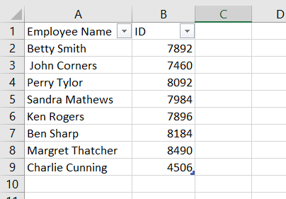
Your table will have all its formatting removed like below:

This method is an excellent way to undo all Excel formatting as a table while maintaining the table. However, one thing to remember is that this method only clears the default table formatting in Excel. If you have any custom formatting, it will remain on your table.

How To Remove Format as Table in Excel by Converting to a Range

Tables are a great tool in Excel, but they can also hinder your workflow, like when using dynamic array formulas that spill. In that case, you may have to remove the table.

Here’s how to clear table formatting in Excel by removing the table completely:

1. Select the entire table or a cell in the table.
2. Click on the “Design” tab that appears in the Excel ribbon.

3. Choose the option “Convert to Range.”

This converts the table back to the normal range, removing the formatting in the process.

Convert To a Range with the Right-Click Menu

Here is how to clear the table format in Excel by right-clicking:

1. Select the table.

2. Right-click on it and choose the “Table” option.

3. Choose the option “Convert to Range.”

With this method, you can also remove the entire table and convert the data back to an ordinary range.

How To Clear All Formatting in a Table

Sometimes, your table may also have custom formatting. Therefore, you may find that when you remove the table formatting, some formatting features still remain.

Let’s assume we added some custom formatting in our example table:

If we clear the table formatting with the step-by-step process above, we’d still be left with the custom formatting.

Here is how to clear all formatting in a table in Excel:

1. Select the entire table.

2. Go to the “Home” tab in the “Editing” section.
3. Click on the drop-down to “Clear.”

4. Choose the option “Clear Formats.”

This will remove all formatting in your table, including any custom formatting and any other formatting unrelated to the table design.

How To Remove a Table in Excel Using VBA

You can also create a script to have Excel remove table formatting. VBA lets you customize functions in Excel and automate tasks.

Here’s how to remove the table format in Excel using VBA:

1. Open the VBA window by going to “Developer” > “Visual Basics.” You can also open it using the keyboard shortcut Alt + F11.

2. In the VBA window, click “Insert” > “Module.”

3. Copy and paste the following Script:

Sub RemoveTableFormat()

Dim wsObj As Worksheet

Dim tableObj As ListObject

For Each wsObj In ActiveWorkbook.Worksheets

    For Each tableObj In wsObj.ListObjects

        tableObj.TableStyle = ""

    Next tableObj

Next wsObj

End Sub

4. Once you have pasted the script, Go to “Run” in the menu and click “Run Sub/Userform.” You can also click the F5 shortcut instead.

This VBA code reads all the tables in your worksheet and automatically sets them to no format. It clears any table format present, including font, colors, and borders, from the data body range, header row, and the total row of the table.

How To Change the Formatting of the Excel Table

Changing the formatting of a table in Excel is pretty simple. When you click on the table, the “Design” tab appears in the Excel ribbon. Here, there are all kinds of formatting options that you can use, including various formatting options in Excel for your table.

Here’s how to change the format of the Excel table:

1. Click on any cell inside the table.
2. Go to the “Design” tab that appears in the Excel ribbon.

3. In the “Design” tab, you’ll find different options to customize the table’s appearance:
   • Table Styles: You can choose from a variety of predefined table styles that come with different formatting options. Click on the drop-down arrow in the “Table Styles” to see the available styles.
     • You can even create your own custom table style by clicking on the option “New Table Style.”

• Table Name: You can change the name of your table in the “Properties” section by typing a new name in the “Table Name” field.

• Header Row: If your table doesn’t have a header row, you can click on the “Header Row” checkbox under the “Table Style Options.” This will treat the first row as the header and apply different formatting to it.

If you want more control over the formatting, you can customize the table manually using the following options:

• Fonts: Click the “Font” option from the “Font” group drop-down to choose a different font for your table data.
• Cell Styles: Click on the “Cell Styles” drop-down in the “Styles” group to apply different predefined styles to your table.
• Fill Color: Click on the “Fill Color” icon in the “Styles” section to change the background color of the selected cells.
• Borders: Click on the “Borders” drop-down in the “Font” section to add or modify cell borders.

Using the choices above, you can make the desired adjustments to the table’s formatting. Formatting can be applied to individual cells, columns, rows, or the entire table. As you change the formatting, the changes are reflected in the table in real-time. When you’re happy with the new formatting, save your Excel worksheet to save the changes.

Wrapping Up

By now, you’ve learned how to remove table formatting in Excel. As you become more accustomed to formatting tables in Excel, you will see how it provides a quick and consistent way to graphically show your data, making it easier for you and your audience to grasp and analyze the information.

Now you’ve completed this Excel “how to remove table formatting” guide, you can extend your learning by using the best Excel courses.

Alternatively, you can skip the learning and use some of our powerful pre-made spreadsheets. Take a look through our premium template library, and don’t forget to use the code “SSP” to get 50% off on all the templates!

Get Premium Templates

Related:

• A Guide to Excel Dashboard + Dashboard Templates
• How To Collapse Rows in Excel in 2 Minutes [Easy Guide]
• How To Use Strikethrough in Excel (5 Easy Ways)