The Google Sheets NOT function is a handy function that lets you negate a logical value or expression. In other words, if the input to the function evaluates to TRUE, the function returns FALSE. Similarly, if the input evaluates to FALSE, the function returns TRUE.
Related: How to Use The NOT Function in Excel
Table of Contents
Syntax for the Google Sheets NOT Function
The syntax for the NOT function is quite simple:
NOT(logical_expression)
Here, logical_expression can be a logical value like TRUE or FALSE, or an entire expression or formula that returns a TRUE or FALSE value. It could also be a reference to a cell containing a logical value.
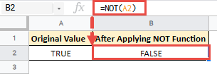
For example, if cell A2 contains the value TRUE, then NOT(A2) will return FALSE.
The NOT formula only accepts one input argument. This makes sense because there’s no logical way to negate more than one logical value together.
Note: The NOT function does accept numbers as input too. In such cases, the function treats any number it receives as a logical TRUE. This includes decimal values too. A zero value, however, is treated as a logical FALSE.
Applications of the Google Sheets NOT Function
Looking at the syntax, the NOT function might look like just a simple function. But it can actually be a pretty good utility function in a number of applications.
Let us take a look at some use cases.
Using NOT Function to Negate a Logical Value
The NOT function can be quite helpful when you want to negate or reverse the outcome of a formula. For example, let’s say we have the following list of people along with their ages:

Say there’s a contest or event and you want to make sure that anyone below the age of 18 is not eligible for a particular task.
To do this you can first find out if a person’s age is less than 18, and if it is, you can simply negate the result to obtain a logical FALSE.
So in cell C2, you can use the formula:
=NOT(B2<18)
Here’s the result you would get for all the cells in column C:
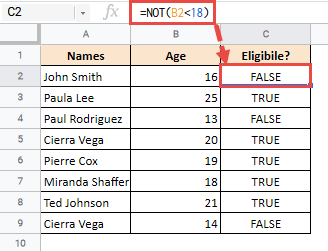
Since John Smith is 16 (which is less than 18), the operation (B2<18) returns a TRUE. The NOT operator then simply reverses the result and returns a FALSE (which means he is not eligible).
The function is also helpful when you want to toggle a result from TRUE to FALSE and back to TRUE each time an event takes place.
Using NOT Function in IF conditions
The NOT function’s most common application is within IF conditions. For example, consider the following data, where there are employees, along with their overtime hours worked:
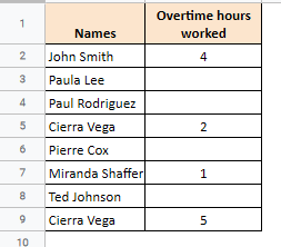
Notice that some of the employees (who did not work overtime) have a blank in the corresponding cell of the ‘Overtime hours worked’ column. We want to calculate the bonus for only those employees who have a non-blank value for overtime hours. For those employees with blank values, we want to display the text “No bonus”.
So in cell C2, you can use the formula:
=IF(NOT(ISBLANK(B2)),B2*25.5,"No Bonus")
Here’s the result you would get for all the cells in column C:
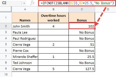
Here we are assuming that for each hour worked overtime, an employee gets $25.5.
Let us break down the formula to understand it:
- The ISBLANK function returns a TRUE if the cell at given cell reference is blank, and a FALSE otherwise. The value is cell A2 is not blank, so the function returns a FALSE.
- Now the NOT function simply reverses the returned value, so NOT(ISBLANK(A2)) returns TRUE.
- The IF function of our formula returns the calculated overtime bonus, B2*25.5 if the condition in its first parameter is TRUE. Otherwise, it returns the text “No Bonus”. In case of cell A2, the first parameter, NOT(ISBLANK(A2)) is TRUE, so the formula returns the value 4*25.5 = 102.
=IF(NOT(ISBLANK(B2)),B2*25.5,"No Bonus")
=IF(NOT(FALSE),B2*25.5,"No Bonus")
=IF(TRUE,B2*25.5,"No Bonus")
=4*25.5
=102
Using NOT Function in Conditional Formatting
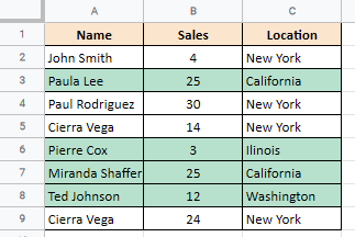
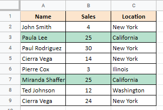
The NOT function is also quite handy when applied to conditional formatting. For example, say you have a list of employees, their sales values and locations:
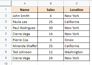
If you want to highlight all the rows where location is not ‘New York’, you can use the NOT function along with conditional formatting as follows:
- Select all the cells in your dataset (cells A2:C9 in our example).
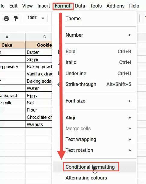
2. From the ‘Format’ menu, select ‘Conditional Formatting’.
3. This will open the ‘Conditional format rules’ sidebar on the right of the window.
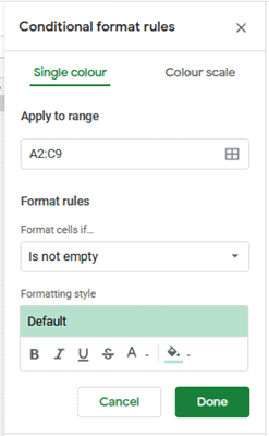
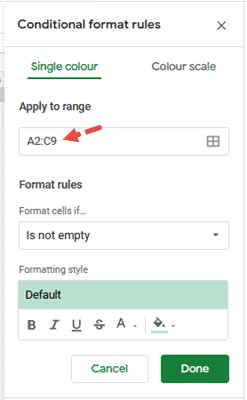
4. In the input box under “Apply to range”, type in the range of cells you want to apply the formatting to. In our example, type the range A2:C9.
5. In the Format rules section, under “Format cells if”, click on the dropdown arrow.
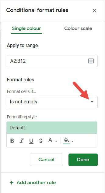
6. Select “Custom formula is” from the dropdown menu.
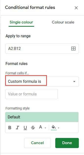
7. You will see an input box below the dropdown list. Type your custom formula there: =NOT($C2=”New York”).
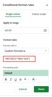
8. Click the Done button.
You will find only those rows highlighted where location is not ”New York”.
Combining NOT with other Logical Operators
You can also combine the NOT operator with other logical operators like AND and NOT.
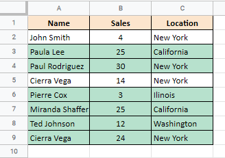
For example, in the previous example, if you wanted all the rows where location is not ‘New York’ and number of Sales is more than 20, you could nest the NOT function inside the AND function as follows:
=AND($B2>20,NOT($C2="New York"))
The above formula returns a TRUE only if both conditions (B2>20) and (NOT(C2=”New York”)) return a TRUE. If even one of these conditions returns a FALSE, then the corresponding row does not get highlighted.
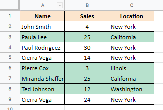
Similarly, if you wanted all the rows where either of the two conditions is true, then you could nest the NOT function inside an OR function as follows:
=OR($B2>20,NOT($C2="New York"))
Here’s the result you get when you apply the above formula to the conditional formatting rule:
An Alternative to the NOT Function
As an alternative to the NOT function, you can use the <> operator in Google Sheets. This operator is basically the reverse of the ‘equal to’ operator (‘=’). So, instead of using the formula NOT($C2=”New York”), you could use the formula =$C2<>”New York”.
Both will give the same result.
In this tutorial we went over the Google Sheets NOT function, along with some ways in which it can be applied. We hope this was helpful in clarifying some of your questions related to the NOT function.


