Array formulas take functions that apply to single cells or ranges and can output the results as a matrix. Using them saves me a ton of time and reduces errors from manual entry.
I understand they can be intimidating when starting. That’s why I’ve put together this helpful array formula Google Sheets guide to walk you through the process.
The crux of this array formula Google Sheets guide is that you can create one using your Windows CTRL + Shift + Enter keyboard shortcut (or Cmd + Shift + Enter on a Mac). Or by using the array formula function.
Table of Contents
What Is an Array?
An array is a mathematical concept derived from the idea of matrices (the plural for matrix). Think of an array as a set of values organized in rows and columns, just like cells in a Google Sheets worksheet.
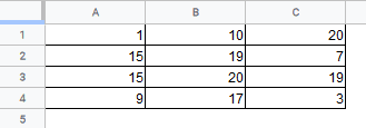
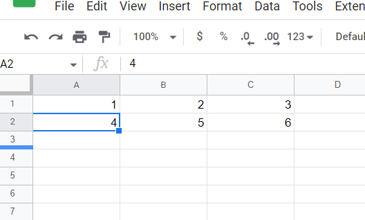
For example, the set of numbers in the range A1 to C4 shown below can be considered an array with four rows and three columns.
An array formula is a formula that is applied to elements of an array like the one shown above. These formulas can perform multiple calculations on the array items and return a single result or a set of results as a new array.
Related: Google Sheets Formulas Cheat Sheet
What Are the Benefits of Using the Array Formula?
- They let you perform multiple calculations at once.
- They let you repeat one or more calculations many times on a selected range of cells.
- Array formulas are helpful when applying a single formula to a whole column or range of cells. Unlike a regular formula, which must be pasted down to the entire column, an array formula lets you skip pasting by displaying results for the whole column in one go.
- Usually, when a computation involves some intermediate results, you need to use some ‘helper’ columns to store them. However, using array formulas lets you skip these intermediate steps and directly display the final result. This gets your work done quickly and keeps your worksheet looking neater.
- The single array formula is expandable. If you change to one place, it expands to the entire range of cells.
- Array formulas are dynamic. They automatically apply to any new Array formula rows introduced into the data range.
Array Formula Google Sheets Syntax
The syntax is the bones of every formula in Google Sheets. And you should know I try to include this for every function I cover.
Here’s the syntax for the array formula function:
=ARRAYFORMULA(array_formula)
As you can see, the array formula function accepts just one parameter, which can be one of the following:
- A reference for a range of cells
- A mathematical expression using cell ranges of the same size
- A function that returns a range of cell values
Creating a Simple Array
The Google Sheets array formula can be complicated for many sheet users. But it doesn’t have to be complicated. Here’s a simple example.
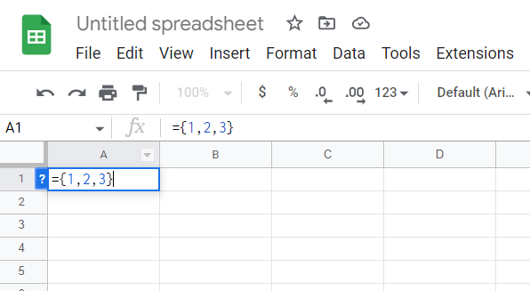
I put the following formula in a cell: ={1, 2, 3}.
The curly brackets are used for the array formula in Google Sheets, displaying the data as an array.
If you press “Enter,” you get the values in three adjacent columns.
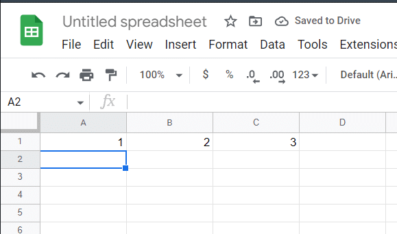
The commas separate the columns, but if you wanted to use rows instead, you would use semicolons (;) instead.
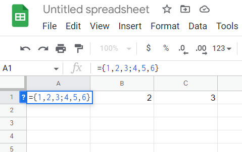
This will give you the values in different rows, one directly below the other.
Hopefully, this was a simple way for you to understand arrays and will contribute to learning how an array formula in Google Sheets works.
Perform Basic Multiplication with Google Sheets Array Functions
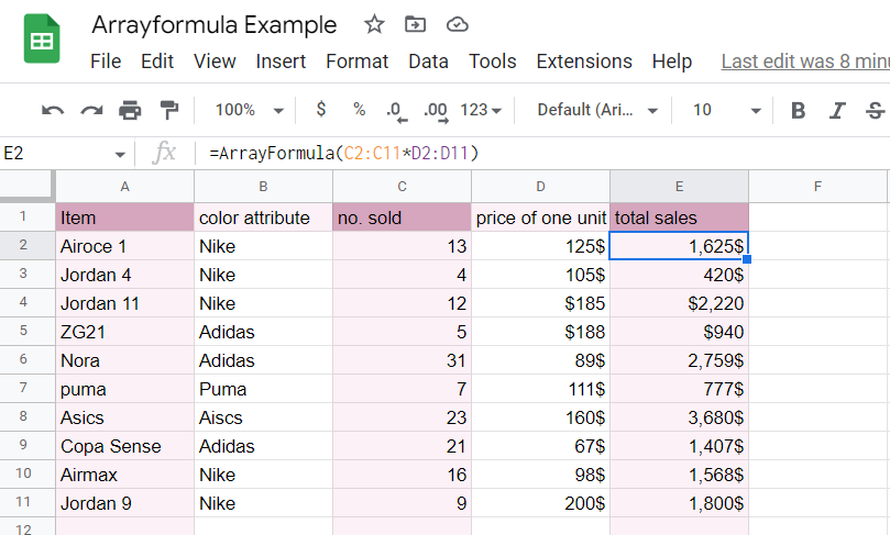
Let’s say you have the following data with the unit cost and quantity sold for each item:
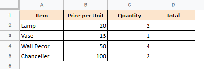
To find the total sales amount for each item, you would normally use the formula =B2*C2 and then use the fill handle to paste the formula into the rest of the cells of column D. This means you have five separate formulas for five items.
You can skip the pasting-down step and directly get the total sales for each item using a single formula as follows:
=ARRAYFORMULA(B2:B5*C2:C5)
As soon as you press the return key after entering the above formula in cell D2, you get the following result:
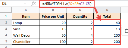
The array formula takes each cell from the range B2:B5 and multiplies with the corresponding cell from the range C2:C5, displaying the result in the corresponding cell of column D (as seen above).
Array Formula Google Sheets Example: Finding Subtotals
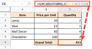
You can also use the SUM function with array formulas to find the overall totals. Here’s the formula that I used in the example image below:
=SUM(ARRAYFORMULA(B2:B5*C2:C5))
How To Use an Array Formula in Google Sheets with Non-Matching Matices
Array formulas provide a great way to perform matrix multiplications. For example, if you have a matrix row named Matrix 1, consisting of 5 rows, and a matrix column named Matrix 2, which is composed of 4 columns, as shown below,
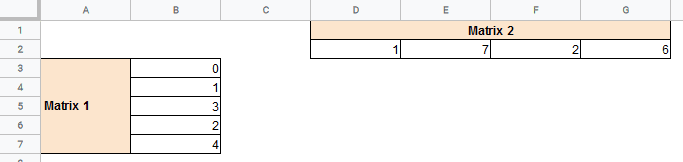
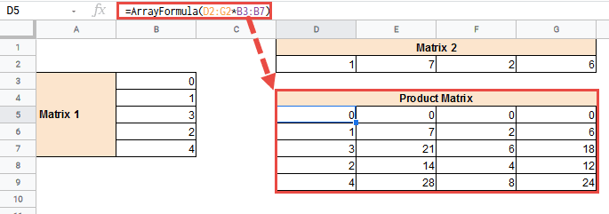
You can find the product of these two matrices using the following array formula:
=ARRAYFORMULA(D2:G2*B3:B7)
As you can see from the screenshot below, this gives a 5×4 matrix containing the product of Matrix 1 and Matrix 2:
Note: This could also be done using the MMULT function in Google Sheets.
Using Array Formula Google Sheets to Concatenate Text
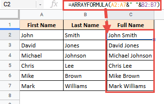
We can also use array formulas to combine columns and concatenate the text. For example, in the screenshot below, we have a list of first and last names.
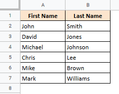
If you want to combine these two columns in one go, you can use the array formula with the concatenation operator as follows:
=ARRAYFORMULA(A2:A7&" "&B2:B7)
When you press the return key after typing in the above formula, you will find all the names and surnames combined with a space in between.
In the same way, you can use the concatenation operator to quickly integrate additional types of text with numbers, dates, or special characters.
Related: How to Combine Cells in Google Sheets [Easy Guide]
Creating an Array Formula in Google Sheets with a Keyboard Shortcut
You can also turn other formulas into array ones using a keyboard shortcut.
Here, you have two options:
- You have to create a new formula
- Click an existing one and press the CTRL+Shift+Enter shortcut (Cmd + Shift + Enter on a Mac) on your keyboard while editing the cell or in the formula bar
Intermediate Array Formula Google Sheets Examples
These next few uses for array formulas might be tricky for new spreadsheet users, but once you have mastered them, they should be easy to use while saving you significant time and effort.
Example Array Formula Google Sheets Worksheet
Click the link to use our example array formula Google Sheets worksheet to help you follow along.
Array Formula Google Sheets With IF Functions
The IF function sets conditions to a formula to return two outcomes: FALSE or TRUE. You can use the Google Sheets array function with the IF function to provide a results matrix.
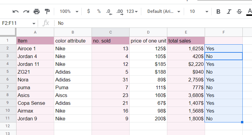
The table below shows the number of shoe sales for different brands. Let’s say I want to find out which shoe brand has sold more than ten pairs of shoes.
Here’s how I’d use an array formula to determine it.
- Select the column where the results will appear, then type the IF formula in the formula bar:
=IF(C2:C11>10,"Yes","No")
- Use the keyboard shortcut Ctrl + Shift+ Enter to input the array formula.
- Use Command + Shift+ Enter for Macbooks.
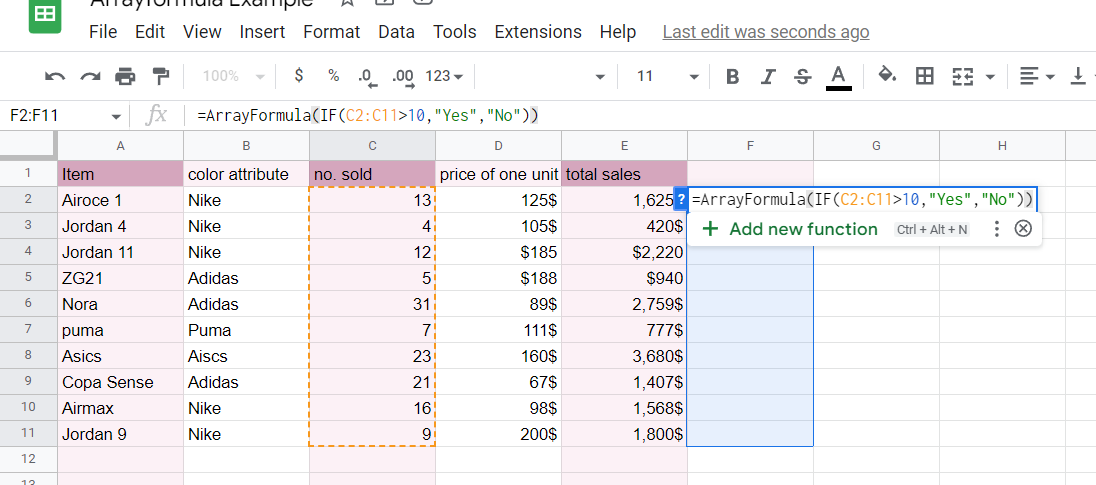
3. Press “Enter” to get the results in the selected column. Shoes that sold more than 10 pairs will be indicated as “Yes” and those with fewer pairs as “No.”
Array Formula Google Sheets VLOOKUP Example
Another way to use the array formula is alongside VLOOKUP. This will enable you to look up data in multiple columns and retrieve the corresponding information.
For example, let’s say I want to find out how many pairs of shoes and the number of sales I made from the shoe stock number 67 (see worksheet below).
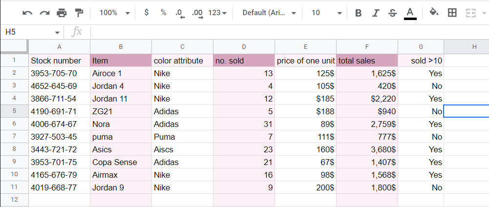
In that case, I would use the VLOOKUP formula on its own. This would retrieve the number of shoes sold according to the stock number using the following formula:
=VLOOKUP("4006-674-67",$A$2:$E$11,4,0)
If I combine it with the array formula Google Sheets function, I can get the values for multiple columns or rows in one go.
For example, if I want to know the multiple values for one stock number like the item, brand, total sales, and sold>10, I would use the following formula:
=ARRAYFORMULA(VLOOKUP($A$2,$A$1:$G$9,{2,3,6,7},FALSE))
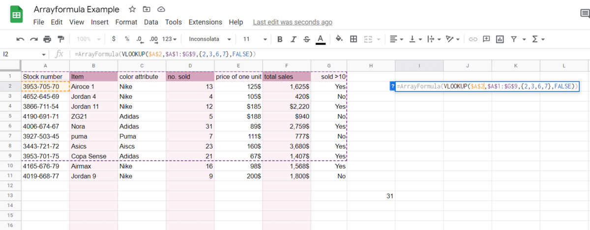
The numbers in the curly brackets represent the columns I want to retrieve the data, i.e., the 2nd, 3rd, 6th, and 7th columns in the range.
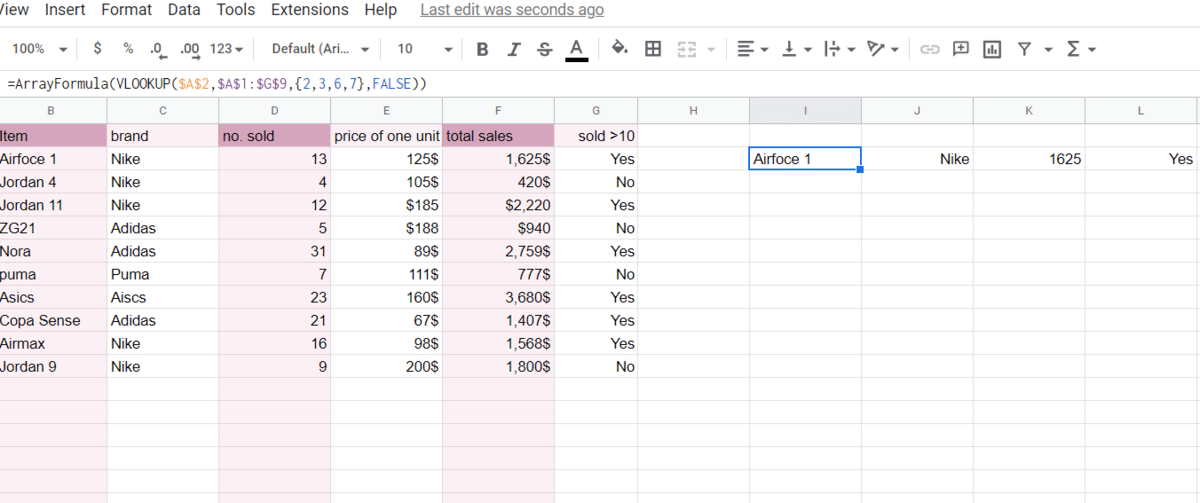
This will return the values from the columns into a new row, as shown below:
Related: How to Pull Information from Another Sheet in Google Sheets
How To Remove Blanks from an Array in Google Sheets
If you combine the array formula function with the blank cells for most functions, you will get the error warning, #REF!
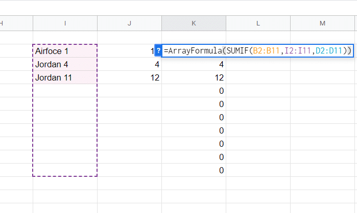
For example, if I used the SUMIF function with the array formula in Google Sheets and there were some extra empty cells, then the formula would return 0 array values for the empty cells.
To remove the extra cells, you can use the IF LEN function by specifying the same ranges as the blank cells in the array formula.
In my example, that would be I2:I11, like so:
=ARRAYFORMULA(IF(LEN(I2:I11),(SUMIF(B2:B11,I2:I11,D2:D11)),))
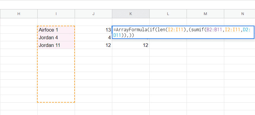
This formula will eliminate all the extra blank cells.
The array formula in sheets will also return 0 for extra blank cells in the criteria region. In this case, to remove the extra blank cells, we can use IF+ISBLANK. This also works in the same way as IF+LEN above.
Eliminate #N/A Errors in Array Formulas
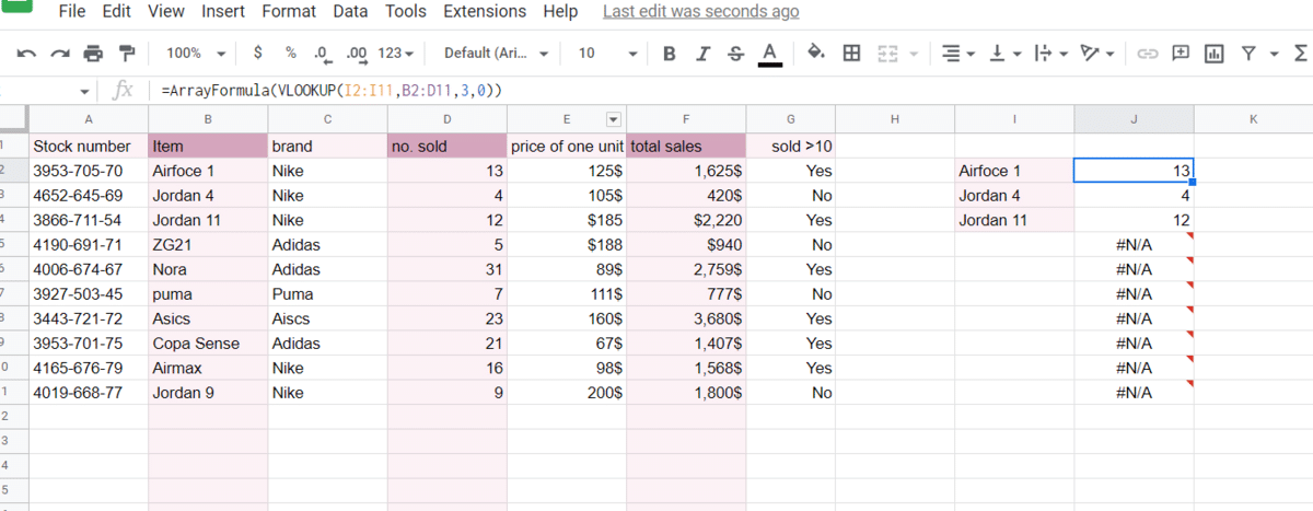
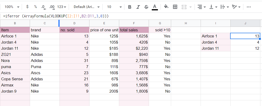
If you use the array formula in Google Sheets with VLOOKUP, it will usually return N/A if there are blank cells. To ignore the blank cells, we can add the IFERROR formula
In such cases, use the following formula:
=ARRAYFORMULA(VLOOKUP(I2:I11,B2:D11,3,0))
Add the IFERROR function before the array formula. This will eliminate the N/A and leave the cells blank.
Using Array Formulas with Aggregation Functions like COUNTIFS and SUMIFS
You can also use array formulas with aggregation functions like SUMIF, SUMIFS, COUNTIF, and COUNTIFS to quickly sum up the values in a range according to one or more conditions.
For example, if you have the following sales amounts item-wise for each store outlet,
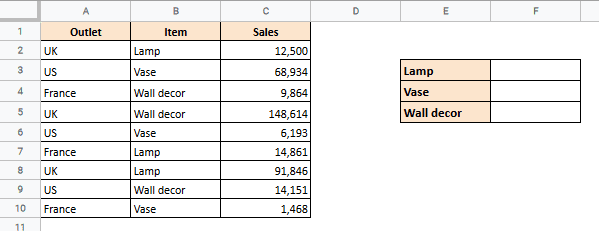
You want to find out the total sales for each item and display these results in cells F3:F5.
If you used a simple SUMIF function for this, you would need to apply the formula three times (one time for each item).
The SUMIF function only allows you to specify one cell in the condition parameter at a time. However, with array formulas, you can specify a range of cells in the condition parameter as follows:
=ARRAYFORMULA(SUMIF(B2:B10,E3:E5,C2:C10))
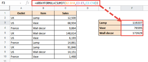
Notice that we specified the range of cells E3:E5 in the second parameter. So we can get the results for all three items at once!
You can also use the COUNTIF function with the array formula similarly if you need to count the number of entries for each item.
Substitute IFS Functions for the & Operator
Applying array formulas with SUMIFS and COUNTIFS functions is slightly more complex. This is because SUMIFS and COUNTIFS return the sum of an array based on multiple conditions, with the result being a single value.
As such, even if you use an array formula with SUMIFS or COUNTIFS functions, it will not make a difference. You will get one result, as shown in the example below:
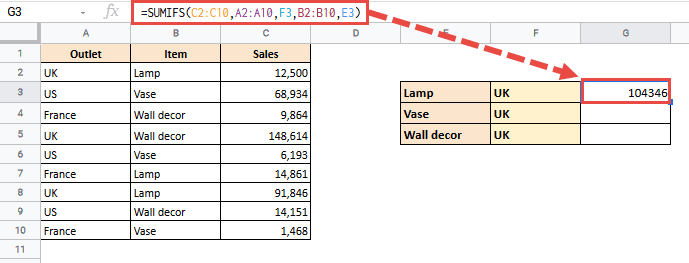
As we can see from the screenshot below, even using Google Sheets array formulas isn’t working.
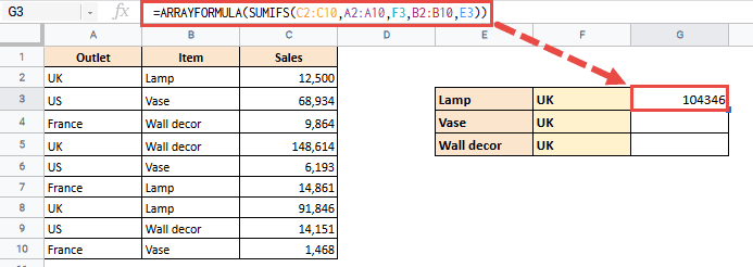
To make this work, improvise your formula using the SUMIF function.
You’ll need to use the Google Sheets array formula and IF functions instead of IFS using the ampersand operator (&) and an array formula!
So, say you only wanted to find the total sales for each item from the UK outlet.
Your formula would then be:
=ARRAYFORMULA(SUMIF(A2:A10&B2:B10,F3:F5&E3:E5,C2:C10))
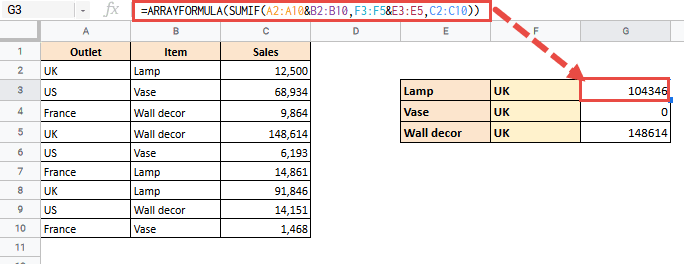
Note that we have two conditions here:
- The item name in column B should match the item name of the corresponding cell in column E
- The Outlet in column A should match the outlet in column F
We combined the ranges and their corresponding criteria using the ampersand operator. After this, we wrapped an array formula around the SUMIF formula.
The SUMIF function now expands its results to the entire column and can even be used to check for multiple criteria.
Video Examples of Array Formulas in Google Sheets
Don’t miss my latest video on how to use array formulas in Google Sheets. Press “play” to watch.
Frequently Asked Questions
Can you Use a horizontal array formula in Google Sheets?
No, there is no way to display the array formula function output horizontally across the page. However, depending on your exact needs, you can use a few workarounds.
The simplest way is to transpose your data using an array formula on the transposed matrix.
Why Use Array Formulas in Google Sheets?
The obvious question that comes to mind is, ‘Why bother’? Array formulas can be intimidating initially, but they are accommodating when used to perform complex calculations like calculating running totals.
Conclusion
In this array formula Google Sheets tutorial, I explained how they work and how versatile these formulas can be. I hope you found my step-by-step guide helpful and easy to follow. If you think I have missed any information, please comment below, and I’ll try to cover it in my next article.
References
- Google. “Share files from Google Drive.” Google Docs Help. Retrieved from https://support.google.com/docs/answer/3093275?hl=en. Accessed March 14, 2024.
- Google. “Stop or change who can share your file in Google Drive.” Google Docs Help. Retrieved from https://support.google.com/docs/answer/3094081?hl=en. Accessed March 14, 2024.