If you work with ever-expanding data (where you keep adding more values in the column or in the row), then sometimes you may have a need to know what’s the last value in the column in Google Sheets.
While you can always scroll down the column and check manually, it’s not an ideal solution.
Thankfully, a little bit of Google sheets formula wizardry can make this possible.
In this tutorial, I will show you how to use a formula to get the last value in the column in Google Sheets(both when you have numbers or text or both in a column).
Table of Contents
Get the Last Number in a Column (when you have numbers)
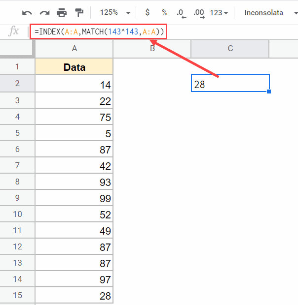
Suppose you have a data set as shown below, and you want to quickly know the last value in this data.
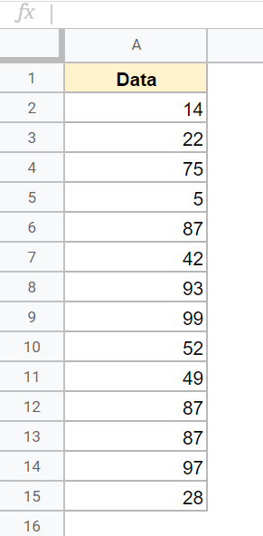
The below formula would do that:
=INDEX(A:A,MATCH(143^143,A:A))
The above formula would give you the right result even if you have blank cells in the dataset
It also only gives you the last numeric value. In case you have a cell that has a text string after the last numeric value, this formula would still give you the numeric value.
How does this formula work?
Now let’s understand the genius in this formula.
I have used the MATCH function to find out the position of the cell that has the last number in the column.
So, if I have a column that has 10 numbers (without any blank cells), the match function would give me 10, which is the position of the last cell with a number in the data set.
With the MATCH function, you can either do an exact-match lookup or an approximate match lookup. When you do an exact match lookup, the MATCH function would only give you the position of the cell in case it finds the exact match.
In this example, I’m using an approximate match as I do not know the last number (and there is also a possibility that there could be repetitions)
Here is the MATCH formula part:
MATCH(143^143,A:A)
The first argument is the lookup value (143^143 in the above formula). This is the value that the match would be looking for in the specified data set.
And the second argument is the range within which the MATCH function is going to look for the first argument. and since we want to find out the last value in the column, I have given the entire column as the lookup range.
Since I have not specified the third argument, it automatically takes that as 1 (which indicates approximate lookup)
The idea in this formula is to have a really large lookup value (143^143 – something which is unlikely to be in the data set) so that the MATCH function is going to go till the end and when it is not able to find this value, it is going to instead return the position of the last filled cell.
In our example data set, the match portion of the formula returns 74, which is the position of the last number in the data set.
Now we can simply use this number within the index function to get the actual value (which is 54 in this example).
Read more: Google Sheets LOOKUP Function
Get the Last Text Value in a Column
Suppose you have a data set as shown below, and you want to quickly know the name of the last person in the list.
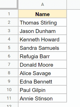
Below is the formula that would do that for you
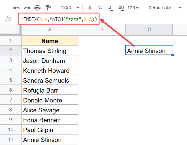
=INDEX(A:A,MATCH("zzzz",A:A))
How does this formula work?
The above formula uses an approximate MATCH formula that goes through the entire list and returns the name that is closest to the lookup value.
In our example, I have used “zzzz” as the lookup value. Since Z is the last alphabet, and ‘zzzz’ is unlikely to be the part of the text in which we are searching, the MATCH function would go till the end, and when it is unable to find anything close to this value it is going to return the position of the last value in the column.
This position value is then used by the index function to return the name in the cell.
Get the Last Value in a Column (that has both Numbers & Text)
In case you have a data set that has a mix of numbers and text values, and you want to find out what’s the last value in the column (be it a number or a text string), you can easily do that as well.
The trick here would be to combine both of these formulas (covered above) and check the position of the last cell that has a number and that has a text string, and return the value where the position value is bigger.
Suppose you have a data set as shown below, and you want to find out the last filled cell in the column.
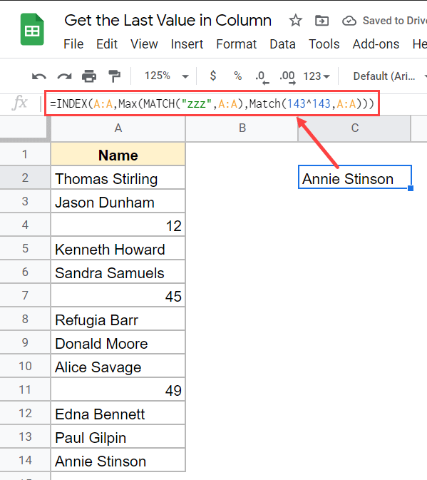
Below is the formula that will do that
=INDEX(A:A,Max(MATCH("zzz",A:A),Match(143^143,A:A)))
How does this formula work?
Since we are dealing with the data set that has both numbers and text values, we need to use two MATCH formulas – one for numbers, and one for text strings.
Both of these match formulas are going to give us a number that will indicate the position of the last filled cell that has a number and the last filled cell that has a text string.
And then we simply use the Max function to find out the position that is bigger and use that in the index function to return the value.
So these are some simple lookup formulas that you can use to get the last value in a column in Google Sheets. The formula you use would depend on whether you have a numeric data set, an alphanumeric data set, or a mix of both.
I hope you found this tutorial useful.
Other Google Sheets tutorial you may also like: