Randomizing data is essential for specific calculations in spreadsheets. But, it can be tricky for some newer users to figure out how to randomize a list in Excel. Luckily, this guide will teach you everything you need to know, from what and why you should randomize lists to learning how. Read on to learn more.
Table of Contents
What Is a Randomized List?
When you randomize a list in Excel, the information order can change every time you refresh a cell or recalculate the values. This method of presenting data can create an unbiased selection.
For example, if you wish to assign a random task to a person in your team. To remain unbiased, you can use Excel randomized list functions to get one person’s name to assign the task to them.
Related: How To Build a Random Number Generator in Google Sheets
Why Randomize a List in Excel?
There are multiple reasons why you may want to randomize data in Excel. Some of the reasons include:
- Creating random samples: Randomizing a list gives you sample values from a large dataset. This is helpful because getting a random value from a large dataset allows you to choose values without any previous bias, making it beneficial for surveys and data analysis.
- Display or presentation purpose: When you randomize Excel lists, it helps you avoid any implicit order that may have existed in the original list, which helps ensure fairness in the presentation of information.
- Shuffling data for simulation: Many people use Excel to play games or create simulations. To keep them interesting, there needs to be an element of randomness. For this, learning how to randomize a list in Excel can help you generate random outcomes. One good example of using this is when playing a card game.
- Anonymity: If you’re looking to share data but you don’t want the viewer to be able to identify any patterns, using a randomized list can be very beneficial. This is particularly useful when you want to ensure the data is anonymous, such as sharing the students’ marks in a class without revealing their names.
Related: How To Randomize a List in Google Sheets
How To Randomize in Excel
There are several randomized Excel list functions. Let’s take a look at them.
How To Randomize a Column in Excel Using RAND
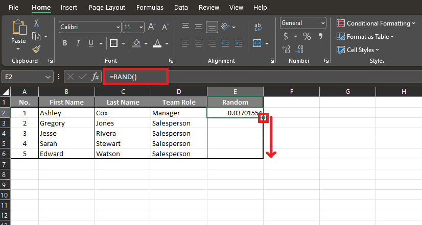
If you want to populate a column with random data, then the RAND function is the best for you. The RAND function can generate a random number between 0 and 1. Let’s take a look at how to create a randomized list using RAND in Excel:
- Open Microsoft Excel and go to the worksheet where you want to create a randomized column.
- Click on the empty cell where you wish to enter the RAND formula.
- Now, enter the RAND formula:
=RAND()
- Press “Enter” to execute the formula.
- To fill the entire column, click on the small dot towards the bottom right part of the cell and drag it downwards to fill the column.
- To randomize the list, we can sort it. To do this, click “Data” in the main header bar.
- Select how you want to view your data from the list of “Sort” options (ascending or descending order). Your data will be displayed in ascending or descending order, depending on your choice.
The RAND formula doesn’t have any parameters, which is why the brackets need to be empty. Depending on your Excel settings, the values in the cell may be recalculated every time the worksheet is updated. If you want to have the same numeric values, copy and paste them back into the cells.
How To Randomize a List in Excel Using RANDBETWEEN
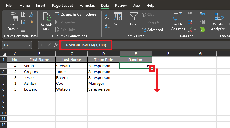
The RANDBETWEEN function is very similar to RAND. However, it returns a random number between a defined number range by the user. Here is how to use RANDBETWEEN to create a random number list:
- Open Microsoft Excel and go to the worksheet where you want to create a randomized column.
- Click on the empty cell where you wish to enter the RANDBETWEEN formula.
- Enter the initial part of the RANDBETWEEN formula:
=RANDBETWEEN(
- Write the first parameter, which is the lowest integer the function can return.
- Add a Comma (,) and write the second parameter, the highest integer that can be returned.
- Add a Closing Bracket ‘ ) ‘ and press “Enter” to execute the formula.
- Fill the entire column or row by clicking and dragging the small dot toward the bottom right part of the cell.
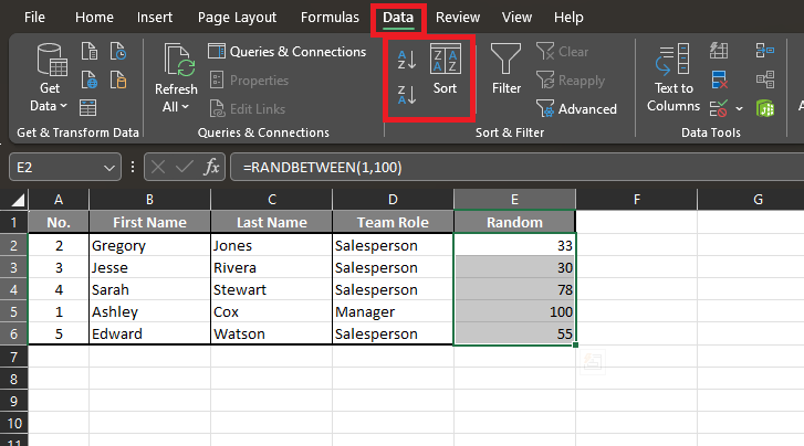
- We can sort the list in ascending or descending order to randomize it. To do this, click “Data” in the main header bar.
- Now, click the appropriate “Sort” options (A-Z or Z-A).
After displaying a confirmation message, the data will be organized according to your chosen sorting order.
How To Randomize a List in Excel Using CHOOSE and RANDBETWEEN
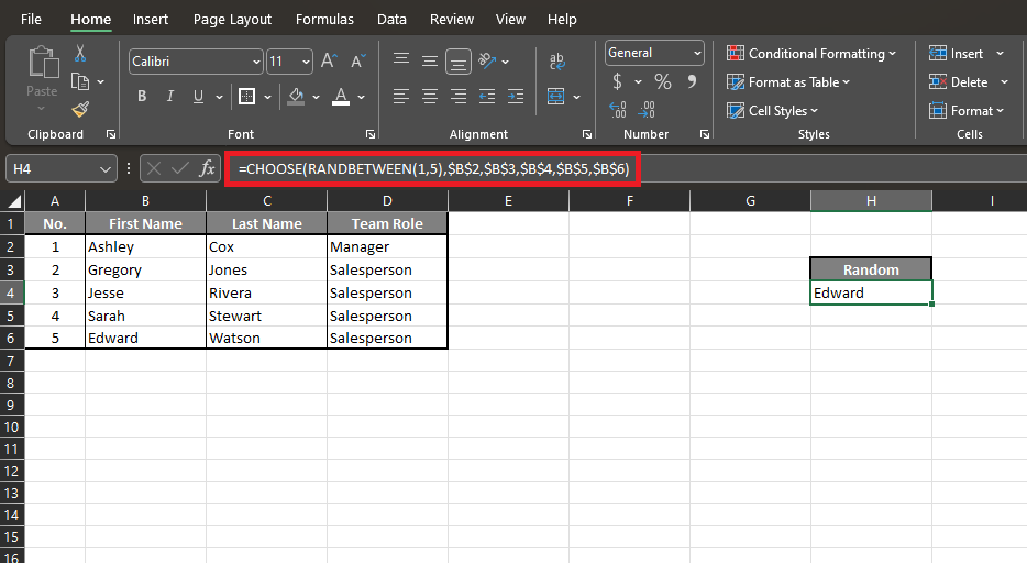
If you don’t want to use the sorting function, an alternative method is to combine the CHOOSE and RANDBETWEEN formulas. If there is only one column that you want to randomize or if you’re randomizing the last column, then you can skip to step 3 (below).
- Open Microsoft Excel and go to the worksheet where you want to create a randomized column.
- Click on the cell next to the main column you wish to randomize to add a new column.
- Enter the initial part of the CHOOSE formula:
=CHOOSE(
- As we nest two formulas, the first parameter will be the RANDBETWEEN formula which is written as:
RANDBETWEEN(
Enter the lower and upper limit parameters separated by a comma and add a Closing Bracket “ ).”
- Now enter the value parameters. These parameters will depend on the number of cells in the column. In the example above, we have five cells with five value parameters. Make sure the values are separated using a Comma (,).
- Add a Closing Bracket “ ) ” to finish the formula and press “Enter” to execute it.
You can execute the nested formula in a single cell or drag-fill it in the entire column if you want to create a longer list. NOTE: This formula will duplicate values.
Related: Excel vs. Google Sheets
Frequently Asked Questions
How To Randomize a Large List in Excel?
The easiest way to randomize an extensive list in Excel is by using the RAND function. The function has no parameters, so enter the formula into the cell by typing =RAND() and pressing “Enter” to execute it.
You can also execute the formula in other cells in a column by using the fill handle towards the of the cell.
Are Duplicates Created When Randomizing a List?
Whether duplicates are created when randomizing the list depends on the process. If you use the RAND function, duplicates won’t be created as the process ensures that each item only appears once.
If you want to have duplicates in the list, use the RANDBETWEEN formula nested in CHOOSE.
Can You Randomize a List in Excel?
You can randomize a list in Microsoft Excel in multiple ways. You can use either the RAND or RANDBETWEEN functions to create a column that you can sort to get a random output each time.
Wrapping Up
In this article, we’ve shown you how to randomize a list in Excel. But that’s just the tip of the iceberg when it comes to learning spreadsheets. You may want to check out our reviews of the best Excel Courses.
Alternatively, check out our premium template library if you want to skip the learning curve and enjoy ready-made robust sheets. Remember to use the code SSP to save 50% too!
Related: